Invertible Constant-Q based on Non-Stationary Gabor frames

07 Feb 2019

A Constant-Q transform is a time/frequency representation where the bins follow a geometric progression. This means that the bins can be chosen to represent the frequencies of the semitones (or fractions of semitones) from an equal-tempered scale. This could be seen as a dimensionality reduction over the Short-Time Fourier transform done in a way that matches the human musical interpretation of frequency.

However, most of the CQ implementations have drawbacks. They are computationally inefficient, lacking C/C++ solutions, and most importantly, not invertible. This makes them unsuitable for applications such as audio modification or synthesis.

Recently we have implemented an invertible CQ algorithm based on Non-Stationary Gabor frames [1]. The NSGConstantQ reference page contains details about the algorithm and the related research.

Below, we will show how to get CQ spectrograms in Essentia and estimate the reconstruction error in terms of SNR.

Standard computation

Here we run the forward and backward transforms on the entire audio file. We are storing some configuration parameters in a dictionary to make sure that the same setup is used for analysis and synthesis. A list of all available parameters can be found in the NSGConstantQ reference page.

from essentia.standard import (MonoLoader, NSGConstantQ, 
    NSGIConstantQ)


# Load an audio file
x = MonoLoader(filename='your/audio/file.wav')()


# Parameters
params = {
          # Backward transform needs to know the signal size.
          'inputSize': x.size,
          'minFrequency': 65.41,
          'maxFrequency': 6000,
          'binsPerOctave': 48,
          # Minimum number of FFT bins per CQ channel.
          'minimumWindow': 128  
         }


# Forward and backward transforms
constantq, dcchannel, nfchannel = NSGConstantQ(**params)(x)
y = NSGIConstantQ(**params)(constantq, dcchannel, nfchannel)

The algorithm generates three outputs: constantq, dcchannel and nfchannel. The reason for this is that the Constant-Q condition is held between the (minFrequency, maxFrequency) range, but the information in the DC and Nyquist channels is also required for perfect reconstruction. We were able to run the analysis/synthesis process at 32x realtime on a 3.4GHz i5-3570 CPU.

Let’s evaluate the quality of the reconstructed signal in terms of SNR:

import numpy as np
from essentia import lin2db


def SNR(r, t, skip=8192):
    """
    r    : reference
    t    : test
    skip : number of samples to skip from the SNR computation
    """
    difference = ((r[skip: -skip] - t[skip: -skip]) ** 2).sum()
    return lin2db((r[skip: -skip] ** 2).sum() / difference)


cq_snr = SNR(x, y)
print('Reconstruction SNR: {:.3f} dB'.format(cq_snr))

Reconstruction SNR: 127.854 dB

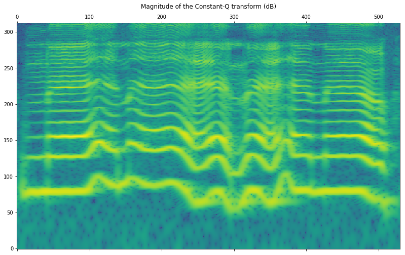
Now let’s plot the transform. Note that as the values are complex, we are only showing their magnitude.

from matplotlib import pyplot as plt
plt.rcParams['figure.figsize'] = (12.0, 8.0)

# Display
plt.matshow(np.log10(np.abs(constantq)),
            origin='lower', aspect='auto')
plt.title('Magnitude of the Constant-Q transform (dB)')
plt.show()

png

Finally, we can listen and compare the original and the reconstructed signals!

Original

from IPython.display import Audio
Audio(x, rate=44100)

Resynthetized

Audio(y, rate=44100)

Framewise computation

Additionally, we have implemented a framewise version of the algorithm that works on half-overlapped frames. This can be useful for very long audio signals that are unsuitable to be processed at once. The algorithm is described in [2]. In this case, we don’t have a dedicated C++ algorithm, but we have implemented a Python wrapper with functions to perform the analysis and synthesis.

import essentia.pytools.spectral as sp

# Forward and backward transforms
cq_frames, dc_frames, nb_frames = sp.nsgcqgram(x, frameSize=4096)
y_frames = sp.nsgicqgram(cq_frames, dc_frames, nb_frames,
                         frameSize=4096)

Reconstruction error in this case:

cq_snr = SNR(x, y_frames[:x.size])
print('Reconstruction SNR: {:.3f} dB'.format(cq_snr))

Reconstruction SNR: 133.596 dB

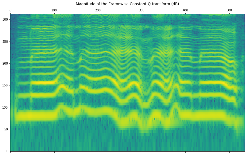
Displaying the framewise transform is slightly more tricky as we have to overlap-add the spectrograms obtained for each frame. To facilitate that we provide a function as shown in the next example. The framewise Constant-Q spectrogram is not supposed to be identical to the standard computation.

# Get the overlap-add version for visualization
cq_overlaped = sp.nsgcq_overlap_add(cq_frames)

plt.matshow(np.log10(np.abs(cq_overlaped)), 
            origin='lower', aspect='auto')
plt.title('Magnitude of the Framewise Constant-Q transform (dB)')
plt.show()

png

Note that it is not possible to synthesize the audio from this overlapped version as we cannot retrieve the analysis frames from it. The synthesis has to be performed from the original list of frames output by the nsgcqgram function.

References

[1] Velasco, G. A., Holighaus, N., Dörfler, M., & Grill, T. (2011). Constructing an invertible constant-Q transform with non-stationary Gabor frames. Proceedings of DAFX11, Paris, 93-99.

[2] Holighaus, N., Dörfler, M., Velasco, G. A., & Grill, T. (2013). A framework for invertible, real-time constant-Q transforms. IEEE Transactions on Audio, Speech, and Language Processing, 21(4), 775-785.

[ news ]

Essentia Labs