Cover song similarity algorithms in Essentia

Cover Song Identification or Music Version Identification is a task of identifying when two musical recordings are derived from the same musical composition. A cover version of a song can be drastically different from the original recording. It may have variations in key, tempo, structure, melody, harmony, timbre, language and lyrics compared to its original version, which makes cover song identification a challenging task [1]. It is typically set as a query-retrieval task where the system retrieves a ranked list of possible covers for a given query song from a reference audio database. ie, the top-most element in the ranked list is the most similar cover song to the query song.

Most of the state-of-the-art cover identification systems undergo the following steps to compute a similarity distance using a pairwise comparison of given music recordings with a query song.

1. Tonal feature extraction using chroma features. This step can be computed using the HPCP or Chromagram algorithms in Essentia.
2. Post-processing of the tonal feature sequences to achieve various invariance to musical facets (eg. Pitch invariance [5]).
3. Computing cross-similarity between a pair of query and reference song tonal features [2, 4].
4. Local sub-sequence alignment to compute the pairwise cover song similarity distance [2, 3, 6].

Recently, we have implemented the following set of algorithms in Essentia to facilitate state-of-the-art cover song identification, providing an optimized open-source implementation for both offline and real-time use-cases. The entire process chain is structured as three different Essentia algorithms in order to provide a maximum level of customization for various types of possible use-cases.

• CrossSimilarityMatrix : Compute euclidean cross-similarity between given two framewise feature arrays with an optional parameter to binarize with a given threshold. This is a generic algorithm that can be used for computing similarity between any given pair of 2D feature arrays. With parameter binarize=True, the output of this algorithm can be used along with local sub-sequence alignment algorithms such as CoverSongSimilarity.

• ChromaChrossSimilarity : This algorithm specifically computes cross-similarity between frame-wise chroma-based features of a query and reference song using cross recurrent plot [2] or OTI-based binary similarity matrix method [4]. With parameter oti=True, the algorithm transposes the pitch of the reference song as of the query song using Optimal Transpose Index [5]. The algorithm always outputs a binary similarity matrix.

• CoverSongSimilarity : Compute cover song similarity distance from an input binary similarity matrix using various alignment constraints [2, 3] of Smith-Waterman local sub-sequence alignment algorithm [6].

In the coming sections, we show how this music similarity and cover song identification algorithms can be used in Essentia in both standard and streaming modes.

Standard mode computation

Step 1

For test example, we selected 3 songs from the covers80 dataset as a query song, true reference song, and a false reference song respectively.

• Query song

• True reference song

• False reference song

Our first step is to load the pre-selected query song and two reference songs using any of the audio loader algorithms in Essentia (here we use MonoLoader. You can check its implementation for more details on how the features are computed). We compute the frame-wise HPCP chroma features for all of these selected songs using the utility function essentia.pytools.spectral.hpcpgram in the Essentia python bindings.

Note: audio files from the covers80 dataset have a sample rate of 32KHz.

import essentia.standard as estd
from essentia.pytools.spectral import hpcpgram

query_filename = "../assests/en_vogue+Funky_Divas+09-Yesterday.mp3"
true_ref_filename = "../assests/beatles+1+11-Yesterday.mp3"
false_ref_filename = "../assests/aerosmith+Live_Bootleg+06-Come_Together.mp3"

# query cover song
query_audio = estd.MonoLoader(filename=query_filename, 
                              sampleRate=32000)()
# true cover
true_cover_audio = estd.MonoLoader(filename=true_ref_filename,       
                                   sampleRate=32000)()
# wrong match
false_cover_audio = estd.MonoLoader(filename=false_ref_filename, 
                                    sampleRate=32000)()

# compute frame-wise hpcp with default params
query_hpcp = hpcpgram(query_audio, 
                      sampleRate=32000)

true_cover_hpcp = hpcpgram(true_cover_audio, 
                           sampleRate=32000)

false_cover_hpcp = hpcpgram(false_cover_audio, 
                            sampleRate=32000)

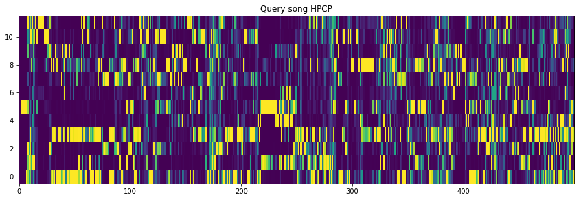
Okay, let’s plot the first 500 frames of HPCP features of the query song.

%matplotlib inline
import matplotlib.pyplot as plt

plt.title("Query song HPCP")
plt.imshow(query_hpcp[:500].T, aspect='auto', origin='lower')

Step 2

The next step is to compute the cross-similarity between the given query and reference song frame-wise HPCP features using ChromaChrossSimilarity algorithm. The algorithm provides two types of methods based on [2] and [4] respectively to compute the aforementioned cross-similarity.

In this case, we have to compute the cross-similarity between the query-true_cover and query-false_cover pairs.

Here oti=True parameter enables the optimal transposition index to introduce pitch invariance among the query and reference song as described in [5].

cross_similarity = estd.ChromaCrossSimilarity(frameStackSize=9, 
                                        frameStackStride=1, 
                                        binarizePercentile=0.095,
                                        oti=True)


true_pair_sim_matrix = cross_similarity(query_hpcp, true_cover_hpcp)

Let’s plot the obtained cross-similarity matrix [2] between the query and true reference cover song frame-wise HPCP features.

plt.xlabel('Yesterday accapella cover')
plt.ylabel('Yesterday - The Beatles')
plt.imshow(true_pair_crp, origin='lower')

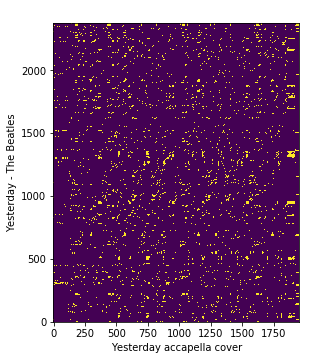
On the above plot, we can see the similarity between each pair of HPCP frames across query and reference songs. ie, The resulting matrix has a shape M x N where M is the number of frames of query song and N is the number of frames of the reference song.

We will call the resulting cross-similarity matrix as query-true_cover for further reference.

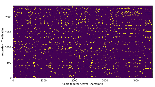
Now, let’s compute the cross-similarity between the query song and false reference cover song HPCP features.

false_pair_sim_matrix = cross_similarity(query_hpcp, false_cover_hpcp)

# plot 
plt.xlabel('Come together cover - Aerosmith')
plt.ylabel('Yesterday - The Beatles')
plt.imshow(false_pair_crp, origin='lower')

We will call the resulting cross-similarity matrix as query-false_cover for further reference.

OR

(Optional)

Alternatively, we can also use the OTI-based binary similarity method as explained in [4] to compute the cross similarity of two given chroma features by enabling the parameter otiBinary=True.

cross_similarity = estd.ChromaCrossSimilarity(frameStackSize=9, 
                                            frameStackStride=1, 
                                            binarizePercentile=0.095,
                                            oti=True,
                                            otiBinary=True)

# for query-true_cover cross-similarity
true_pair_sim_matrix = csm_oti(query_hpcp, true_cover_hpcp)

# for query-false_cover cross-similarity
false_pair_sim_matrix = cross_similarity(query_hpcp, false_cover_hpcp)

Step 3

The last step is to compute an cover song similarity distance between both query-true_cover and query-false_cover pairs using a local sub-sequence alignment algorithm designed for the cover song identification task. CoverSongSimilarity algorithm in Essentia provides two alignment constraints of the Smith-Waterman algorithm [6] based on [2] and [3]. We can switch between these methods using the alignmentType parameter. With parameter distanceType, we can also specify if we want a symmetric (maximum value in the alignment score matrix) or asymmetric cover similarity distance (normalized by the length of reference song). Please refer to the documentation and references for more details.

Let’s compute the cover song similarity distance between true cover song pairs using the method described in [2].

score_matrix, distance = estd.CoverSongSimilarity(disOnset=0.5, 
                                            disExtension=0.5, 
                                            alignmentType='serra09',
                                            distanceType='asymmetric')
                                            (true_pair_crp)

In the above-given example, score_matrix is the Smith-Waterman alignment scoring matrix. Now, let’s plot the obtained score matrix and cover song similarity distance.

plt.title('Cover song similarity distance: %s' % distance)
plt.xlabel('Yesterday accapella cover')
plt.ylabel('Yesterday - The Beatles')
plt.imshow(score_matrix, origin='lower')

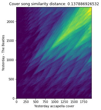
From the plot, we can clearly see long and densely closer diagonals which give us the notion of closer similarity between the query and reference song as expected.

Now, let’s compute the cover song similarity distance between false cover song pairs.

score_matrix, distance = estd.CoverSongSimilarity(disOnset=0.5, 
                                            disExtension=0.5, 
                                            alignmentType='serra09',
                                            distanceType='asymmetric')
                                            (false_pair_crp)

# plot
plt.title('Cover song similarity distance: %s' % distance)
plt.ylabel('Yesterday accapella cover')
plt.xlabel('Come together cover - Aerosmith')
plt.imshow(score_matrix, origin='lower')

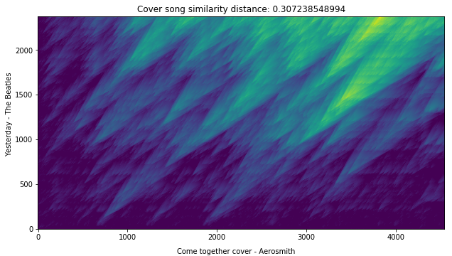
Voila! We can see that the cover similarity distance is quite low for the actual cover song pairs as expected.

Streaming mode computation

We can also compute the same similarity measures using the Essentia streaming mode, which suits real-time applications. The following code block shows a simple example of the workflow where we stream a query song audio file to compute the cover song similarity distance between a pre-computed reference song HPCP feature in real-time.

import essentia.streaming as estr
from essentia import array, run, Pool

query_filename = "../assests/en_vogue+Funky_Divas+09-Yesterday.mp3"

# Let's instantiate all the required essentia streaming algorithms

audio = estr.MonoLoader(filename=query_filename, sampleRate=32000)
  
frame_cutter = estr.FrameCutter(frameSize=4096, hopSize=2048)

windowing = estr.Windowing(type="blackmanharris62")

spectrum  = estr.Spectrum();

peak = estr.SpectralPeaks(sampleRate=32000)

whitening = estr.SpectralWhitening(maxFrequency=3500,
                                sampleRate=32000);

hpcp = estr.HPCP(sampleRate=32000,
                 minFrequency=100,
                 maxFrequency=3500,
                 size=12);

# Create an instance of streaming ChromaCrossSimilarity algorithm
# With parameter `referenceFeature`, 
# we can pass the pre-computed reference song chroma features.
# In this case, we use the pre-computed HPCP feature 
# of the 'true_cover_song'.
# With parameter `oti`, we can tranpose the pitch 
# of the reference song HPCP feature
# to an given OTI [5] (if it's known before hand).
# By default we set `oti=0`
sim_matrix = estr.ChromaCrossSimilarity(
                referenceFeature=true_cover_hpcp,
                oti=0)

# Create an instance of the cover song similarity alignment algorithm 
# 'pipeDistance=True' stdout distance values for each input stream
alignment = estr.CoverSongSimilarity(pipeDistance=True)

# essentia Pool instance (python dict like object) to aggregrate the outputs  
pool = Pool()

# Connect all the required algorithms in a essentia streaming network
# ie., connecting inputs and outputs of the algorithms 
# in the required workflow and order
audio.audio >> frame_cutter.signal
frame_cutter.frame >> windowing.frame
windowing.frame >> spectrum.frame
spectrum.spectrum >> peak.spectrum
spectrum.spectrum >> whitening.spectrum
peak.magnitudes >> whitening.magnitudes
peak.frequencies >> whitening.frequencies
peak.frequencies >> hpcp.frequencies 
whitening.magnitudes >> hpcp.magnitudes
hpcp.hpcp >> sim_matrix.queryFeature
sim_matrix.csm >> alignment.inputArray
alignment.scoreMatrix >> (pool, 'scoreMatrix')
alignment.distance >> (pool, 'distance')

# Run the algorithm network
run(audio)
# This process will stdout the cover song similarity distance 
# for every input stream in realtime.
# It also aggregrates the Smith-Waterman alignment score matrix 
# and cover song similarity distance for every accumulating 
# input audio stream in an essentia pool instance (similar to a python dict) 
# which can be accessed after the end of the stream.

# Now, let's check the final cover song similarity distance value 
# computed at the last input stream.
print(pool['distance'][-1])

References

[1] Joan Serrà. Identification of Versions of the Same Musical Composition by Processing Audio Descriptions. PhD thesis, Universitat Pompeu Fabra, Spain, 2011.

[2] Serra, J., Serra, X., & Andrzejak, R. G. (2009). Cross recurrence quantification for cover song identification.New Journal of Physics.

[3] Chen, N., Li, W., & Xiao, H. (2017). Fusing similarity functions for cover song identification. Multimedia Tools and Applications.

[4] Serra, Joan, et al. Chroma binary similarity and local alignment applied to cover song identification. IEEE Transactions on Audio, Speech, and Language Processing 16.6 (2008).

[5] Serra, J., Gómez, E., & Herrera, P. (2008). Transposing chroma representations to a common key, IEEE Conference on The Use of Symbols to Represent Music and Multimedia Objects.

[6] Smith-Waterman algorithm (Wikipedia, https://en.wikipedia.org/wiki/Smith%E2%80%93Waterman_algorithm).

[ news ]