The complete list of models supported in Essentia along with their vocabulary is available on Essentia’s site, and the experimental results and implementation details are available in the paper [1] and the official repository.
According to the authors, the fsd-sinet-vgg42-tlpf_aps-1 model featuring TLPF and APS obtained the best evaluation metrics.
Additionally, fsd-sinet-vgg41-tlpf-1 is a lighter architecture using TLPF intended for reduced computational cost.
As an example, let’s analyze a field recording and observe the model’s predictions.
Note: Remember to update Essentia before running the code.
These models make predictions each 0.5 seconds by default.
Internally, they operate on 10 ms frames, and the number of frames to jump (50 by default) can be controlled with the patchHopSize parameter.
Additionally, the models can be configured to return embeddings instead of activations by setting the parameter output="model/global_max_pooling1d/Max".
The following code visualizes the top activations using matplotlib and the model’s metadata:
importjsonimportmatplotlib.pyplotaspltimportnumpyasnpdeftop_from_average(data,top_n=10):av=np.mean(data,axis=0)sorting=np.argsort(av)[::-1]returnsorting[:top_n],[av[i]foriinsorting]# Read the metadata
metadata_file="fsd-sinet-vgg42-tlpf_aps-1.json"metadata=json.load(open(metadata_file,"r"))labels=metadata["classes"]# Compute the top-n labels and predictions
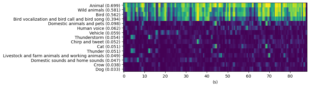
top_n,averages=top_from_average(predictions,top_n=15)top_labels=[labels[i]foriintop_n]top_labels_with_av=[f"{label} ({av:.3f})"forlabel,avinzip(top_labels,averages)]top_predictions=np.array([predictions[i,:]foriintop_n])# Generate plots and improve formatting
matfig=plt.figure(figsize=(8,3))plt.matshow(top_predictions,fignum=matfig.number,aspect="auto")plt.yticks(np.arange(len(top_labels_with_av)),top_labels_with_av)locs,_=plt.xticks()ticks=np.array(locs//2).astype("int")plt.xticks(locs[1:-1],ticks[1:-1])plt.tick_params(bottom=True,top=False,labelbottom=True,labeltop=False)plt.xlabel("(s)")plt.savefig("activations.png",bbox_inches='tight')
As can be seen, the model detects the intermittent bird sounds and some of the backgrounds sounds are identified as Vehicle or Thunder with lower probabilities.
In this post, we demonstrate how to use TensorFlow models in Essentia for real-time music audio annotation. Find more information about the available models and the introduction to our TensorFlow wrapper in our previous posts.
Real-time constraints are a common requirement for many applications that involve digital audio signal processing and analysis in a wide variety of contexts, and deployment scenarios, and the approaches relying on deep learning should be no exception. For this reason, we have equipped Essentia with algorithms that support inference with deep learning models in real-time.
This real-time capability, however, ultimately relies on the complexity of the models and the computational resources at hand. Some of our models currently available for download are lightweight enough to perform real-time predictions with a CPU on a regular laptop, and we have prepared a demo to show you this!
Our demo utilizes SoundCard to read the computer audio loopback, capturing all audio that is playing on the system, such as coming from a local music player application or a web browser (e.g., from Youtube). It is streamed to Essentia in real-time for the prediction of music tags that can be associated with the audio.
We use a pre-trained auto-tagging model based on the MusiCNN architecture, introduced in our previous post, adapted to operate on small one-second chunks of audio.
This process does not require any extra training, but it reduces the performance of the model a bit. A mel-spectrogram of each chunk serves as an input to the model.
The video below shows a moving mel-spectrogram window on the left and the resulting tag activations on the right.
One cool feature of our collection of models is that the same processing chain can be applied to the transfer learning classifiers based on the MusiCNN architecture. These classifier models were obtaining by retraining the last layer of the MusiCNN auto-tagging model, and therefore we can use all of them simultaneously without any computational overhead. In the next video, you can see the real-time predictions of the classifiers trained for detecting aggressive and happy moods, danceability, and voice activity in music.
You are welcome to try this demo on your own, and of course, it can be adapted to many other TensorFlow models for sound and music audio annotation.
We envision many promising applications of the real-time inference functionality in Essentia. For example, we can use it for recognition of relevant semantic characteristics in the context of online music streaming and radio broadcasts. In music production tools, it can help to generate valuable real-time feedback based on “smarter” audio analysis and foster development of powerful audio effects using deep learning.
Note: the models were updated on 2020-07-08 due to a new name convention and some upgrades. See the full CHANGELOG for more details.
In our last post, we introduced the TensorFlow wrapper for Essentia. It can be used with virtually any TensorFlow model and here we present a collection of models we supply with Essentia out of the box.
First, we prepared a set of pre-trained auto-tagging models achieving state
of-the-art performance. Then, we used those models as feature extractors to
generate a set of transfer learning classifiers trained on our in-house
datasets.
Along with the models we provide helper algorithms that allow performing predictions in just a couple of lines. Also, we include C++ extractors that could be built statically to use as standalone executables.
Supplied models
Auto-tagging models
Our auto-tagging models were pre-trained as part of Jordi Pons’ Ph.D. Thesis [1]. They were trained on two research datasets, MSD and MTT, to predict top 50 tags therein. Check the original repository for more details about the training process.
The following table shows the available architectures and the datasets used for training. For every model, its complexity is reported in terms of the number of trainable parameters. The models were trained and evaluated using the standardized train/test splits proposed for these datasets in research. The performance of the models is indicated in terms of ROC-AUC and PR-AUC obtained on the test splits. Additionally, the table provides download links for the models and README files containing the output labels, the name of the relevant layers and some details about the training datasets.
In transfer learning, a model is first trained on a source task (typically with a greater amount of available data) to leverage the obtained knowledge in a smaller target task. In this case, we considered the aforementioned MusiCNN models and a big VGG-like (VGGish) model as source tasks. As target tasks, we considered our in-house classification datasets listed below. We use the penultimate layer of the source task models as feature extractors for small classifiers consisting of two fully connected layers.
The following tables present all trained classifiers in genre, mood and miscellaneous task categories. For each classifier, its source task name represents a combination of the architecture and the training dataset used. Its complexity is reported in terms of the number of trainable parameters. The performance of each model is measured in terms of normalized accuracy (Acc.) in a 5-fold cross-validation experiment conducted before the final classifier model was trained on all data.
MusiCNN is a musically-motivated Convolutional Neural Network. It uses vertical and horizontal convolutional filters aiming to capture timbral and temporal patterns, respectively. The model contains 6 layers and 790k parameters.
VGG is an architecture from computer vision based on a deep stack of commonly used 3x3 convolutional filters. It contains 5 layers with 128 filters each. Batch normalization and dropout are applied before each layer. The model has 605k trainable parameters. We are using the implementation by Jordi Pons.
VGGish [2, 3] follows the configuration E from the original implementation for computer vision, with the difference that the number of output units is set to 3087. This model has 62 million parameters.
Datasets details
MSD contains 200k tracks from the train set of the publicly available Million Song Dataset (MSD) annotated by tags from Last.fm. Only top 50 tags are used.
MTT contains 25k tracks from Magnatune with tags by human annotators. Only top 50 tags are used.
AudioSet contains 1.8 million audio clips from Youtube annotated with the AudioSet taxonomy, not specific to music.
MTG in-house datasets are a collection of small, highly curated datasets used for training classifiers. A set of SVM classifiers based on these datasets is also available.
Dataset
Classes
Size
genre_dortmund
alternative, blues, electronic, folkcountry, funksoulrnb, jazz, pop, raphiphop, rock
1820
genre_gtzan
blues, classic, country, disco, hip hop, jazz, metal, pop, reggae, rock
1000
genre_rosamerica
classic, dance, hip hop, jazz, pop, rhythm and blues, rock, speech
400
genre_electronic
ambient, dnb, house, techno, trance
250
mood_acoustic
acoustic, not acoustic
321
mood_electronic
electronic, not electronic
332
mood_aggressive
aggressive, not aggressive
280
mood_relaxed
not relaxed, relaxed
446
mood_happy
happy, not happy
302
mood_sad
not sad, sad
230
mood_party
not party, party
349
danceability
danceable, not dancable
306
voice_instrumental
voice, instrumental
1000
gender
female, male
3311
tonal_atonal
atonal, tonal
345
Helper algorithms
Algorithms for MusiCNN and VGG based models:
TensorflowInputMusiCNN. Computes mel-bands with a particular parametrization specific
to MusiCNN based models.
TensorflowPredictMusiCNN. Makes predictions using MusiCNN models.
Algorithms for VGGish based models:
TensorflowInputVGGish. Computes mel-bands with a particular parametrization specific
to VGGish based models.
TensorflowPredictVGGish. Makes predictions using VGGish models.
Usage examples
Let’s exemplify some use cases.
Auto-tagging
In this case, we are replicating the example of our previous post. With the new algorithms, the code is reduced to just a couple of lines!
importnumpyasnpfromessentia.standardimport*msd_labels=['rock','pop','alternative','indie','electronic','female vocalists','dance','00s','alternative rock','jazz','beautiful','metal','chillout','male vocalists','classic rock','soul','indie rock','Mellow','electronica','80s','folk','90s','chill','instrumental','punk','oldies','blues','hard rock','ambient','acoustic','experimental','female vocalist','guitar','Hip-Hop','70s','party','country','easy listening','sexy','catchy','funk','electro','heavy metal','Progressive rock','60s','rnb','indie pop','sad','House','happy']# Our models take audio streams at 16kHz
sr=16000# Instantiate a MonoLoader and run it in the same line
audio=MonoLoader(filename='/your/amazong/song.wav',sampleRate=sr)()# Instatiate the tagger and pass it the audio
predictions=TensorflowPredictMusiCNN(graphFilename='msd-musicnn-1.pb')(audio)# Retrieve the top_n tags
top_n=3# The shape of the predictions matrix is [n_patches, n_labels]
# Take advantage of NumPy to average them over the time axis
averaged_predictions=np.mean(predictions,axis=0)# Sort the predictions and get the top N
fori,linenumerate(averaged_predictions.argsort()[-top_n:][::-1],1):print('{}: {}'.format(i,msd_labels[l]))
1: electronic
2: chillout
3: ambient
Classification
In this example, we are using our genre_rosamerica classifier based on the VGGish embeddings. Note that this time we are using TensorflowPredictVGGish instead of TensorflowPredictMusiCNN so that the model is fed with the correct input features.
importnumpyasnpfromessentia.standardimport*labels=['classic','dance','hip hop','jazz','pop','rnb','rock','speech']sr=16000audio=MonoLoader(filename='/your/amazing/song.wav',sampleRate=sr)()predictions=TensorflowPredictVGGish(graphFilename='genre_rosamerica-vggish-audioset-1.pb')(audio)# Average predictions over the time axis
predictions=np.mean(predictions,axis=0)order=predictions.argsort()[::-1]foriinorder:print('{}: {:.3f}'.format(labels[i],predictions[i]))
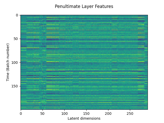
As the last example, let’s use one of the models as a feature extractor by retrieving the output of the penultimate layer. This is done by setting the output parameter in the predictor algorithm.
A list of the supported output layers is available in the README files supplied with the models.
fromessentia.standardimportMonoLoader,TensorflowPredictMusiCNNsr=16000audio=MonoLoader(filename='/your/amazing/song.wav',sampleRate=sr)()# Retrieve the output of the penultimate layer
penultimate_layer=TensorflowPredictMusiCNN(graphFilename='msd-musicnn-1.pb',output='model/dense/BiasAdd')(audio)
The following plot shows how these features look like:
References
[1] Pons, J., & Serra, X. (2019). musicnn: Pre-trained convolutional neural networks for music audio tagging. arXiv preprint arXiv:1909.06654.
[2] Gemmeke, J. et. al., AudioSet: An ontology and human-labelled dataset for audio events, ICASSP 2017.
[3] Hershey, S. et. al., CNN Architectures for Large-Scale Audio Classification, ICASSP 2017
Audio Signal Processing and Music Information Retrieval evolve very fast and there is a tendency to rely more and more on Deep Learning solutions. For this reason, we see the necessity to support these solutions in Essentia to keep up with the state of the art. After having worked on this for the past months, we are delighted to present you a new set of algorithms and models that employ TensorFlow in Essentia. These algorithms are suited for inference tasks and offer the flexibility of use, easy extensibility, and (in some cases) real-time inference.
In this post, we will show how to install Essentia with TensorFlow support, how to prepare your pre-trained models, and how to use them for prediction in both streaming and standard modes. See our next post for the list of all models available in Essentia.
For now, the installation steps are only available for Linux. Nevertheless, we are planning to support other platforms too.
Installing Essentia with TensorFlow
From PyPI wheels
For convenience, we have built special Python 3 Linux wheels for using Essentia with TensorFlow that can be installed with pip. These wheels include the required shared library for TensorFlow 1.15. Note that a pip version ≥19.3 is required (you should be fine creating a new virtualenv environment as it will contain an appropriate pip version).
pip3 install essentia-tensorflow
Building Essentia from source
A more flexible option is to build the library from source. This way we have the freedom to choose the TensorFlow version to use, which may be useful to ensure compatibility for certain models. In this case, we keep using version 1.15.
As an example, let’s try to use MusiCNN, a pre-trained auto-tagging model based on Convolutional Neural Networks (CNNs). There are versions trained on different datasets. In this case, we will consider the model relying on the subset of Million Song Dataset annotated by last.fm tags that was trained on the top 50 tags.
Here we are reproducing this blogpost as a demonstration of how simple it is to incorporate a model into our framework.
All we need is to get the model in Protobuf format (we provide more pre-made models on our webpage) and obtain its labels and the names of the input and output layers. If the names of the layers are not supplied there are plenty of online resources explaining how to inspect the model to get those.
One of the keys to making predictions faster is the use of our C++ extractor. Essentia’s algorithm for mel-spectrogram offers parameters that make it possible to reproduce the features from most of the well-known audio analysis libraries. In this case, we are reproducing the training features that were computed with Librosa:
First of all, we instantiate the required algorithms using the streaming mode of Essentia:
fromessentia.streamingimport*fromessentiaimportPool,runfilename='your/amazing/song.mp3'# Algorithms for mel-spectrogram computation
audio=MonoLoader(filename=filename,sampleRate=sampleRate)fc=FrameCutter(frameSize=frameSize,hopSize=hopSize)w=Windowing(normalized=False)spec=Spectrum()mel=MelBands(numberBands=numberBands,sampleRate=sampleRate,highFrequencyBound=sampleRate//2,inputSize=frameSize//2+1,weighting=weighting,normalize=normalize,warpingFormula=warpingFormula)# Algorithms for logarithmic compression of mel-spectrograms
shift=UnaryOperator(shift=1,scale=10000)comp=UnaryOperator(type='log10')# This algorithm cuts the mel-spectrograms into patches
# according to the model's input size and stores them in a data
# type compatible with TensorFlow
vtt=VectorRealToTensor(shape=[1,1,patchSize,numberBands])# Auxiliar algorithm to store tensors into pools
ttp=TensorToPool(namespace=input_layer)# The core TensorFlow wrapper algorithm operates on pools
# to accept a variable number of inputs and outputs
tfp=TensorflowPredict(graphFilename=modelName,inputs=[input_layer],outputs=[output_layer])# Algorithms to retrieve the predictions from the wrapper
ptt=PoolToTensor(namespace=output_layer)ttv=TensorToVectorReal()# Another pool to store output predictions
pool=Pool()
Then we connect all the algorithms:
audio.audio>>fc.signalfc.frame>>w.framew.frame>>spec.framespec.spectrum>>mel.spectrummel.bands>>shift.arrayshift.array>>comp.arraycomp.array>>vtt.framevtt.tensor>>ttp.tensorttp.pool>>tfp.poolIntfp.poolOut>>ptt.poolptt.tensor>>ttv.tensorttv.frame>>(pool,output_layer)# Store mel-spectrograms to reuse them later in this tutorial
comp.array>>(pool,"melbands")
Now we can run the Network and measure the prediction time:
The new algorithms are also available in the standard mode where they can be called as regular functions. This provides more flexibility in order to integrate them with a 3rd-party code in Python:
In this example we’ll take advantage of the previously computed mel-spectrograms:
bands=pool['melbands']discard=bands.shape[0]%patchSize# Would not fit into the patch.
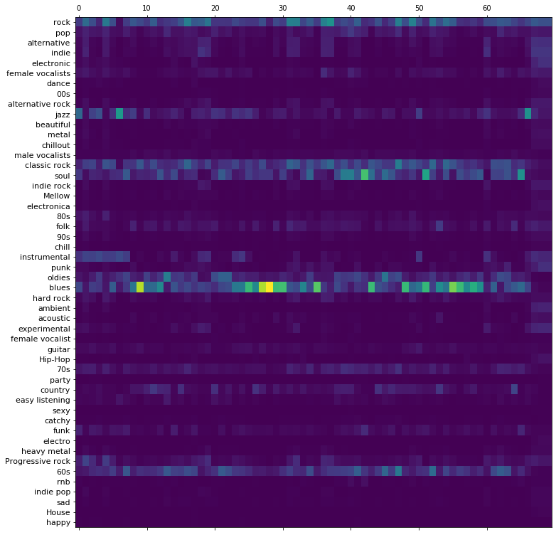
bands=np.reshape(bands[:-discard,:],[-1,patchSize,numberBands])batch=np.expand_dims(bands,2)in_pool.set('model/Placeholder',batch)out_pool=predict(in_pool)print('Most predominant tags:')fori,linenumerate(np.mean(out_pool[output_layer].squeeze(),axis=0).argsort()[-3:][::-1],1):print('{}: {}'.format(i,msd_labels[l]))
Most predominant tags:
1: blues
2: rock
3: classic rock
How fast is it?
Let’s compare with the original Python implementation:
Prediction time: 10.38s
Computing spectrogram (w/ librosa) and tags (w/ tensorflow)..
done!
[barry_white-you_heart_and_soul.mp3] Top3 tags:
 - blues
 - rock
 - classic rock
Which is more than two times the time it took in Essentia. Great!
Using TensorFlow frozen models
In order to maximize efficiency, we only support frozen TensorFlow models. By freezing a model its variables are converted into constant values allowing for some optimizations.
Frozen models are easy to generate given a TensorFlow architecture and its weights. In our case, we have used the following script where our architecture is defined on an external method DEFINE_YOUR_ARCHITECTURE() and the weights are loaded from a CHECKPOINT_FOLDER/:
importtensorflowastfmodel_fol='YOUR/MODEL/FOLDER/'output_graph='YOUR_MODEL_FILE.pb'withtf.name_scope('model'):DEFINE_YOUR_ARCHITECTURE()sess=tf.Session()sess.run(tf.global_variables_initializer())saver=tf.train.Saver()saver.restore(sess,'CHECKPOINT_FOLDER/')gd=sess.graph.as_graph_def()fornodeingd.node:ifnode.op=='RefSwitch':node.op='Switch'forindexinrange(len(node.input)):if'moving_'innode.input[index]:node.input[index]=node.input[index]+'/read'elifnode.op=='AssignSub':node.op='Sub'if'use_locking'innode.attr:delnode.attr['use_locking']elifnode.op=='AssignAdd':node.op='Add'if'use_locking'innode.attr:delnode.attr['use_locking']elifnode.op=='Assign':node.op='Identity'if'use_locking'innode.attr:delnode.attr['use_locking']if'validate_shape'innode.attr:delnode.attr['validate_shape']iflen(node.input)==2:node.input[0]=node.input[1]delnode.input[1]node_names=[n.nameforningd.node]output_graph_def=tf.graph_util.convert_variables_to_constants(sess,gd,node_names)# Write to Protobuf format
tf.io.write_graph(output_graph_def,model_fol,output_graph,as_text=False)sess.close()
Cover Song Identification or Music Version Identification is a task of identifying when two musical recordings are derived from the same musical composition. A cover version of a song can be drastically different from the original recording. It may have variations in key, tempo, structure, melody, harmony, timbre, language and lyrics compared to its original version, which makes cover song identification a challenging task [1]. It is typically set as a query-retrieval task where the system retrieves a ranked list of possible covers for a given query song from a reference audio database. ie, the top-most element in the ranked list is the most similar cover song to the query song.
Most of the state-of-the-art cover identification systems undergo the following steps to compute a similarity distance using a pairwise comparison of given music recordings with a query song.
Tonal feature extraction using chroma features. This step can be computed using the HPCP or Chromagram algorithms in Essentia.
Post-processing of the tonal feature sequences to achieve various invariance to musical facets (eg. Pitch invariance [5]).
Computing cross-similarity between a pair of query and reference song tonal features [2, 4].
Local sub-sequence alignment to compute the pairwise cover song similarity distance [2, 3, 6].
Recently, we have implemented the following set of algorithms in Essentia to facilitate state-of-the-art cover song identification, providing an optimized open-source implementation for both offline and real-time use-cases. The entire process chain is structured as three different Essentia algorithms in order to provide a maximum level of customization for various types of possible use-cases.
CrossSimilarityMatrix : Compute euclidean cross-similarity between given two framewise feature arrays with an optional parameter to binarize with a given threshold. This is a generic algorithm that can be used for computing similarity between any given pair of 2D feature arrays. With parameter binarize=True, the output of this algorithm can be used along with local sub-sequence alignment algorithms such as CoverSongSimilarity.
ChromaChrossSimilarity : This algorithm specifically computes cross-similarity between frame-wise chroma-based features of a query and reference song using cross recurrent plot [2] or OTI-based binary similarity matrix method [4]. With parameter oti=True, the algorithm transposes the pitch of the reference song as of the query song using Optimal Transpose Index [5]. The algorithm always outputs a binary similarity matrix.
CoverSongSimilarity : Compute cover song similarity distance from an input binary similarity matrix using various alignment constraints [2, 3] of Smith-Waterman local sub-sequence alignment algorithm [6].
In the coming sections, we show how this music similarity and cover song identification algorithms can be used in Essentia in both standard and streaming modes.
Standard mode computation
Step 1
For test example, we selected 3 songs from the covers80 dataset as a query song, true reference song, and a false reference song respectively.
Query song
True reference song
False reference song
Our first step is to load the pre-selected query song and two reference songs using any of the audio loader algorithms in Essentia (here we use MonoLoader. You can check its implementation for more details on how the features are computed). We compute the frame-wise HPCP chroma features for all of these selected songs using the utility function essentia.pytools.spectral.hpcpgram in the Essentia python bindings.
Note: audio files from the covers80 dataset have a sample rate of 32KHz.
importessentia.standardasestdfromessentia.pytools.spectralimporthpcpgramquery_filename="../assests/en_vogue+Funky_Divas+09-Yesterday.mp3"true_ref_filename="../assests/beatles+1+11-Yesterday.mp3"false_ref_filename="../assests/aerosmith+Live_Bootleg+06-Come_Together.mp3"# query cover song
query_audio=estd.MonoLoader(filename=query_filename,sampleRate=32000)()# true cover
true_cover_audio=estd.MonoLoader(filename=true_ref_filename,sampleRate=32000)()# wrong match
false_cover_audio=estd.MonoLoader(filename=false_ref_filename,sampleRate=32000)()# compute frame-wise hpcp with default params
query_hpcp=hpcpgram(query_audio,sampleRate=32000)true_cover_hpcp=hpcpgram(true_cover_audio,sampleRate=32000)false_cover_hpcp=hpcpgram(false_cover_audio,sampleRate=32000)
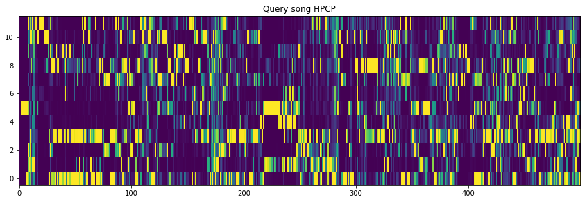
Okay, let’s plot the first 500 frames of HPCP features of the query song.
%matplotlibinlineimportmatplotlib.pyplotaspltplt.title("Query song HPCP")plt.imshow(query_hpcp[:500].T,aspect='auto',origin='lower')
Step 2
The next step is to compute the cross-similarity between the given query and reference song frame-wise HPCP features using ChromaChrossSimilarity algorithm. The algorithm provides two types of methods based on [2] and [4] respectively to compute the aforementioned cross-similarity.
In this case, we have to compute the cross-similarity between the query-true_cover and query-false_cover pairs.
Here oti=True parameter enables the optimal transposition index to introduce pitch invariance among the query and reference song as described in [5].
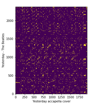
Let’s plot the obtained cross-similarity matrix [2] between the query and true reference cover song frame-wise HPCP features.
plt.xlabel('Yesterday accapella cover')plt.ylabel('Yesterday - The Beatles')plt.imshow(true_pair_crp,origin='lower')
On the above plot, we can see the similarity between each pair of HPCP frames across query and reference songs. ie, The resulting matrix has a shape M x N where M is the number of frames of query song and N is the number of frames of the reference song.
We will call the resulting cross-similarity matrix as query-true_cover for further reference.
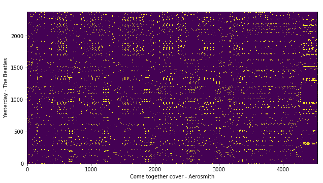
Now, let’s compute the cross-similarity between the query song and false reference cover song HPCP features.
false_pair_sim_matrix=cross_similarity(query_hpcp,false_cover_hpcp)# plot
plt.xlabel('Come together cover - Aerosmith')plt.ylabel('Yesterday - The Beatles')plt.imshow(false_pair_crp,origin='lower')
We will call the resulting cross-similarity matrix as query-false_cover for further reference.
OR
(Optional)
Alternatively, we can also use the OTI-based binary similarity method as explained in [4] to compute the cross similarity of two given chroma features by enabling the parameter otiBinary=True.
cross_similarity=estd.ChromaCrossSimilarity(frameStackSize=9,frameStackStride=1,binarizePercentile=0.095,oti=True,otiBinary=True)# for query-true_cover cross-similarity
true_pair_sim_matrix=csm_oti(query_hpcp,true_cover_hpcp)# for query-false_cover cross-similarity
false_pair_sim_matrix=cross_similarity(query_hpcp,false_cover_hpcp)
Step 3
The last step is to compute an cover song similarity distance between both query-true_cover and query-false_cover pairs using a local sub-sequence alignment algorithm designed for the cover song identification task. CoverSongSimilarity algorithm in Essentia provides two alignment constraints of the Smith-Waterman algorithm [6] based on [2] and [3]. We can switch between these methods using the alignmentType parameter. With parameter distanceType, we can also specify if we want a symmetric (maximum value in the alignment score matrix) or asymmetric cover similarity distance (normalized by the length of reference song).
Please refer to the documentation and references for more details.
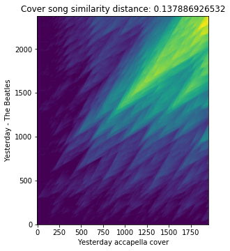
Let’s compute the cover song similarity distance between true cover song pairs using the method described in [2].
In the above-given example, score_matrix is the Smith-Waterman alignment scoring matrix. Now, let’s plot the obtained score matrix and cover song similarity distance.
plt.title('Cover song similarity distance: %s'%distance)plt.xlabel('Yesterday accapella cover')plt.ylabel('Yesterday - The Beatles')plt.imshow(score_matrix,origin='lower')
From the plot, we can clearly see long and densely closer diagonals which give us the notion of closer similarity between the query and reference song as expected.
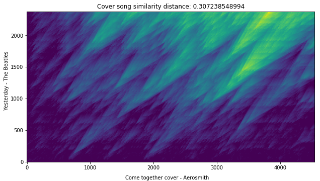
Now, let’s compute the cover song similarity distance between false cover song pairs.
score_matrix,distance=estd.CoverSongSimilarity(disOnset=0.5,disExtension=0.5,alignmentType='serra09',distanceType='asymmetric')(false_pair_crp)# plot
plt.title('Cover song similarity distance: %s'%distance)plt.ylabel('Yesterday accapella cover')plt.xlabel('Come together cover - Aerosmith')plt.imshow(score_matrix,origin='lower')
Voila! We can see that the cover similarity distance is quite low for the actual cover song pairs as expected.
Streaming mode computation
We can also compute the same similarity measures using the Essentia streaming mode, which suits real-time applications. The following code block shows a simple example of the workflow where we stream a query song audio file to compute the cover song similarity distance between a pre-computed reference song HPCP feature in real-time.
importessentia.streamingasestrfromessentiaimportarray,run,Poolquery_filename="../assests/en_vogue+Funky_Divas+09-Yesterday.mp3"# Let's instantiate all the required essentia streaming algorithms
audio=estr.MonoLoader(filename=query_filename,sampleRate=32000)frame_cutter=estr.FrameCutter(frameSize=4096,hopSize=2048)windowing=estr.Windowing(type="blackmanharris62")spectrum=estr.Spectrum();peak=estr.SpectralPeaks(sampleRate=32000)whitening=estr.SpectralWhitening(maxFrequency=3500,sampleRate=32000);hpcp=estr.HPCP(sampleRate=32000,minFrequency=100,maxFrequency=3500,size=12);# Create an instance of streaming ChromaCrossSimilarity algorithm
# With parameter `referenceFeature`,
# we can pass the pre-computed reference song chroma features.
# In this case, we use the pre-computed HPCP feature
# of the 'true_cover_song'.
# With parameter `oti`, we can tranpose the pitch
# of the reference song HPCP feature
# to an given OTI [5] (if it's known before hand).
# By default we set `oti=0`
sim_matrix=estr.ChromaCrossSimilarity(referenceFeature=true_cover_hpcp,oti=0)# Create an instance of the cover song similarity alignment algorithm
# 'pipeDistance=True' stdout distance values for each input stream
alignment=estr.CoverSongSimilarity(pipeDistance=True)# essentia Pool instance (python dict like object) to aggregrate the outputs
pool=Pool()# Connect all the required algorithms in a essentia streaming network
# ie., connecting inputs and outputs of the algorithms
# in the required workflow and order
audio.audio>>frame_cutter.signalframe_cutter.frame>>windowing.framewindowing.frame>>spectrum.framespectrum.spectrum>>peak.spectrumspectrum.spectrum>>whitening.spectrumpeak.magnitudes>>whitening.magnitudespeak.frequencies>>whitening.frequenciespeak.frequencies>>hpcp.frequencieswhitening.magnitudes>>hpcp.magnitudeshpcp.hpcp>>sim_matrix.queryFeaturesim_matrix.csm>>alignment.inputArrayalignment.scoreMatrix>>(pool,'scoreMatrix')alignment.distance>>(pool,'distance')# Run the algorithm network
run(audio)# This process will stdout the cover song similarity distance
# for every input stream in realtime.
# It also aggregrates the Smith-Waterman alignment score matrix
# and cover song similarity distance for every accumulating
# input audio stream in an essentia pool instance (similar to a python dict)
# which can be accessed after the end of the stream.
# Now, let's check the final cover song similarity distance value
# computed at the last input stream.
print(pool['distance'][-1])
References
[1] Joan Serrà. Identification of Versions of the Same Musical Composition by Processing Audio Descriptions. PhD thesis, Universitat Pompeu Fabra, Spain, 2011.
[2] Serra, J., Serra, X., & Andrzejak, R. G. (2009). Cross recurrence quantification for cover song identification.New Journal of Physics.
[3] Chen, N., Li, W., & Xiao, H. (2017). Fusing similarity functions for cover song identification. Multimedia Tools and Applications.
[4] Serra, Joan, et al. Chroma binary similarity and local alignment applied to cover song identification. IEEE Transactions on Audio, Speech, and Language Processing 16.6 (2008).
[5] Serra, J., Gómez, E., & Herrera, P. (2008). Transposing chroma representations to a common key, IEEE Conference on The Use of Symbols to Represent Music and Multimedia Objects.
A Constant-Q transform is a time/frequency representation where the bins follow a geometric progression. This means that the bins can be chosen to represent the frequencies of the semitones (or fractions of semitones) from an equal-tempered scale. This could be seen as a dimensionality reduction over the Short-Time Fourier transform done in a way that matches the human musical interpretation of frequency.
However, most of the CQ implementations have drawbacks. They are computationally inefficient, lacking C/C++ solutions, and most importantly, not invertible. This makes them unsuitable for applications such as audio modification or synthesis.
Recently we have implemented an invertible CQ algorithm based on Non-Stationary Gabor frames [1]. The NSGConstantQ reference page contains details about the algorithm and the related research.
Below, we will show how to get CQ spectrograms in Essentia and estimate the reconstruction error in terms of SNR.
Standard computation
Here we run the forward and backward transforms on the entire audio file. We are storing some configuration parameters in a dictionary to make sure that the same setup is used for analysis and synthesis. A list of all available parameters can be found in the NSGConstantQ reference page.
fromessentia.standardimport(MonoLoader,NSGConstantQ,NSGIConstantQ)# Load an audio file
x=MonoLoader(filename='your/audio/file.wav')()# Parameters
params={# Backward transform needs to know the signal size.
'inputSize':x.size,'minFrequency':65.41,'maxFrequency':6000,'binsPerOctave':48,# Minimum number of FFT bins per CQ channel.
'minimumWindow':128}# Forward and backward transforms
constantq,dcchannel,nfchannel=NSGConstantQ(**params)(x)y=NSGIConstantQ(**params)(constantq,dcchannel,nfchannel)
The algorithm generates three outputs: constantq, dcchannel and nfchannel. The reason for this is that the Constant-Q condition is held between the (minFrequency, maxFrequency) range, but the information in the DC and Nyquist channels is also required for perfect reconstruction. We were able to run the analysis/synthesis process at 32x realtime on a 3.4GHz i5-3570 CPU.
Let’s evaluate the quality of the reconstructed signal in terms of SNR:
importnumpyasnpfromessentiaimportlin2dbdefSNR(r,t,skip=8192):"""
r : reference
t : test
skip : number of samples to skip from the SNR computation
"""difference=((r[skip:-skip]-t[skip:-skip])**2).sum()returnlin2db((r[skip:-skip]**2).sum()/difference)cq_snr=SNR(x,y)print('Reconstruction SNR: {:.3f} dB'.format(cq_snr))
Reconstruction SNR: 127.854 dB
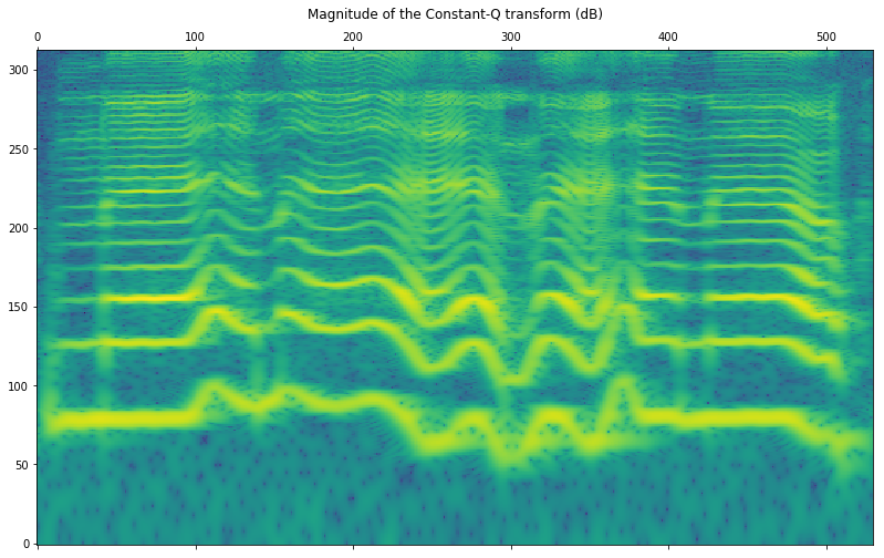
Now let’s plot the transform. Note that as the values are complex, we are only showing their magnitude.
frommatplotlibimportpyplotaspltplt.rcParams['figure.figsize']=(12.0,8.0)# Display
plt.matshow(np.log10(np.abs(constantq)),origin='lower',aspect='auto')plt.title('Magnitude of the Constant-Q transform (dB)')plt.show()
Finally, we can listen and compare the original and the reconstructed signals!
Original
fromIPython.displayimportAudioAudio(x,rate=44100)
Resynthetized
Audio(y,rate=44100)
Framewise computation
Additionally, we have implemented a framewise version of the algorithm that works on half-overlapped frames. This can be useful for very long audio signals that are unsuitable to be processed at once. The algorithm is described in [2]. In this case, we don’t have a dedicated C++ algorithm, but we have implemented a Python wrapper with functions to perform the analysis and synthesis.
importessentia.pytools.spectralassp# Forward and backward transforms
cq_frames,dc_frames,nb_frames=sp.nsgcqgram(x,frameSize=4096)y_frames=sp.nsgicqgram(cq_frames,dc_frames,nb_frames,frameSize=4096)
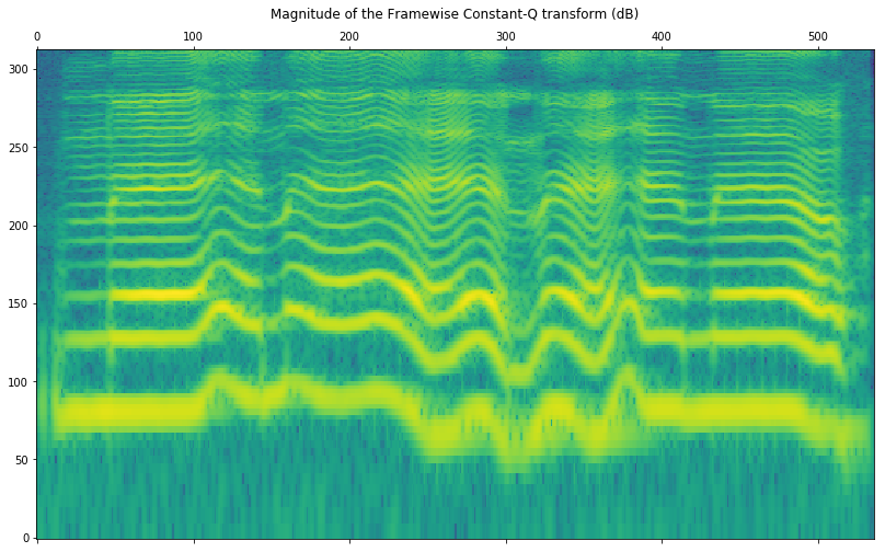
Displaying the framewise transform is slightly more tricky as we have to overlap-add the spectrograms obtained for each frame. To facilitate that we provide a function as shown in the next example. The framewise Constant-Q spectrogram is not supposed to be identical to the standard computation.
# Get the overlap-add version for visualization
cq_overlaped=sp.nsgcq_overlap_add(cq_frames)plt.matshow(np.log10(np.abs(cq_overlaped)),origin='lower',aspect='auto')plt.title('Magnitude of the Framewise Constant-Q transform (dB)')plt.show()
Note that it is not possible to synthesize the audio from this overlapped version as we cannot retrieve the analysis frames from it. The synthesis has to be performed from the original list of frames output by the nsgcqgram function.
References
[1] Velasco, G. A., Holighaus, N., Dörfler, M., & Grill, T. (2011). Constructing an invertible constant-Q transform with non-stationary Gabor frames. Proceedings of DAFX11, Paris, 93-99.
[2] Holighaus, N., Dörfler, M., Velasco, G. A., & Grill, T. (2013). A framework for invertible, real-time constant-Q transforms. IEEE Transactions on Audio, Speech, and Language Processing, 21(4), 775-785.
As we are gradually expanding Essentia with new functionality, we have added a new algorithm for computation of audio fingerprints, the Chromaprinter. Technically, it is a wrapper of Chromaprint library which you will need to install to be able to use Chromaprinter.
The fingerprints computed with Chromaprinter can be used to query the AcoustID database for track metadata. Check a few examples of how Chromaprinter can be used in Python here. To start using this algorithm now, build the latest Essentia code from the master branch.
We now host images on docker hub containing Essenta, the python bindings, and all pre-built examples. This means that you can run Essentia on Linux, Mac, or Windows without having to compile it yourself.
We publish 6 variations, on three different operating systems: Ubuntu 16.04 LTS, Ubuntu 17.10, Debian 9.0 Stretch, and a python 2 and python 3 variation for each OS.
See the documentation for further information on how to run an example or python file using these images.
These images can also be used as a base image for your own docker projects if you want Essentia available.
Working towards the next Essentia release, we have updated our cepstral features. The updates include:
Support for extracting MFCCs ‘the htk way’ (python example).
In literature there are two common MFCCs ‘standards’ differing in some parameters and the mel-scale computation itself: the Slaney way (Auditory toolbox) and the htk way (chapter 5.4 from htk book).
See a python notebook for a comparison with mfcc extracted with librosa and with htk.
Support for inverting the computed MFCCs back to spectral (mel) domain (python example).
The first MFCC coefficients are standard for describing singing voice timbre. The MFCC feature vector however does not represent the singing voice well visually. Instead, it is a common practice to invert the first 12-15 MFCC coefficients back to mel-bands domain for visualization. We have ported invmelfcc.m as explained here.
Keeping Essentia in constant development, we are glad to announce that Essentia 2.1 beta3 has been recently released. It is a preliminary version of the forthcoming 2.1 release and is the version recommended to install. This version includes a very significant amount of new algorithms, updates, bug-fixes and documentation improvements. The full list of changes can be seen here.
We are now hosting static binaries for a number command-line extractors, originally developed as examples of how Essentia can be used in applications. These tools make it easy to compute some descriptors and store them to a file given an audio file as an input (therefore, called “extractors”) without any need to install Essentia library itself.
In particular these extractors can:
compute a large set of spectral, time-domain, rhythm, tonal and high-level descriptors
compute MFCC frames
extract pitch of a predominant melody using MELODIA algorithm
extract pitch for a monophonic signal using YinFFT algorithm
extract beats
Notably, two extractors, specifically designed for AcousticBrainz and Freesound projects are included. They include large sets of features and are designed for batch processing large amounts of audio files.
See description of the extractors in the official documentation. Specifically, here you will find details about our music extractor.
We are very excited to announce the AcousticBrainz, a new collaboration project between MusicBrainz community and the Music Technology Group, that uses the power of music analysis done by Essentia to build a large-scale open content database of music.
The goal of the project is to crowd source acoustic information for all music in the world and to make it available to the public, providing a massive database of information about music for music technology researchers and open-source hackers. The project relies on Essentia for extracting acoustic characteristics of music, including low-level spectral information, rhythm, keys, scales, and much more, and automatic annotation by genres, moods, and instrumentation.
Since the first public announcement a month ago, the project has gained more than 1.2 million of analysed tracks. The possibility to bring audio analysis on the large scale while having all the data and tools in open access, and the instant feedback from the users, makes this project an exciting opportunity to explore the opportunities of the state-of-the-art music analysis tools and improve them. See more details about the project on the official AcousticBrainz website.
This new version includes high-level classifier models and a number of minor updates:
Added pre-trained high-level classifier models for genres, moods, rhythm and instrumentation (to be used with streaming_extractor_archivemusicextractor, see accuracies here)
Fixed scheduler in streaming mode
Fixed compilation with clang/libc++/c++11
PitchYinFFT now supports parabolic interpolation
Updated Vamp plugin
Updated documentation and tutorials
Minor bugfixes, more unittests, etc.
Please, compile it, use it and give us feedback!!! As usual, we are looking forward for your ideas and suggestions!
Essentia was presented at the International Society for Music Information Retrieval Conference (ISMIR 2013) that took take place from November 4th to the 8th 2013 in Curitiba (Brazil). The article presented is available from here.
Essentia wins the Open-Source Software Competition of ACM Multimedia 2013, the worldwide premier multimedia conference that took place in Barcelona from October 21st to 25th 2013.
The ACM Multimedia Open-Source Software Competition celebrates the invaluable contribution of researchers and software developers who advance the field by providing the community with implementations of codecs, middleware, frameworks, toolkits, libraries, applications, and other multimedia software. The criteria for judging all submissions include broad applicability and potential impact, novelty, technical depth, demo suitability, and other miscellaneous factors (e.g., maturity, popularity, student-led, no dependence on closed source, etc.).
The article on Essentia presented at ACM Multimedia is available from here.
Today, June 27th 2013, Essentia becomes Open Source Software and we start distributing it using the Affero-GPLv3 license (also available under proprietary license upon request).
In the last few months we have been working hard in the code to make a major upgrade of the existing code and we will continue improving it and adding more functionalities. We encourage everyone to use it, test it, contribute to it, and help make it better than what already is. You can find the source code in the github repository: https://github.com/MTG/essentia. There you can find all the documentation, complementary information, and you can download everything.
We have also opened the Gaia library (under the same license terms), which complements Essentia for indexing and similarity computation tasks. It is available at: https://github.com/MTG/gaia.
Over the years many people have contributed to Essentia, but we specially recognize the work of Nicolas Wack, who was its main developer for many years at the MTG and who has always supported the idea of opening it. We have many plans to promote and exploit Essentia. It is a great tool and we all can do big things with it. Please, compile it, use it and give us feedback!!!