Python for audio processing#
All code-related materials in this tutorial are based in Python. There are several relevant courses and learning materials you may refer to for learning the basics of Python for ASP. We want to highlight the course in Coursera on Audio Signal Processing for Music Applications and AudioLabs-Erlangen FMP Notebooks.
In this section we provide a brief overview of the very basics of Python for digital processing of audio signals, hoping that it serves as a useful entry point to this tutorials for readers that do not have a lot of experience on that particular topic. If you are familiar with the said topic, this section may still be useful since relevant tools for this topic are showcased.
Note
Bear in mind that this is not a complete introduction to ASP: we are just trying to provide an overview of how we process and extract information from audio signals in this tutorial using Python. For a deep introduction the ASP and MIR please refer to the linked tutorials in the paragraph above.
Discretizing audio signals#
In a real-world scenario, sound is produced by pressure waves, air vibrations that are processed by our ears and converted into what we hear. From a computational point of view, we have to convert these signals into a measurable representation that a machine is able to read and process. In other words, these signals must be digitalized or discretizing the continuous (or analog) sound into a representable sequence of values. See an example in Fig. 1.
Fig. 1 We represent the continuous signal using a sequence of points (image from sonimbus.com).#
Note
The time-step between points is given by the sampling frequency (or sampling rate), which is a variable given in Hertz (Hz), and that indicates us how many samples per seconds we are using to represent the continuous signal. Common values for music signals are 8kHz, 16kHz, 22.05kHz, 44.1kHz, and finally 48kHz.
The important thing here is: these captured discrete values can be easily loaded and used in a Python project, normally represented as an array of data points. We can use several different libraries and pipelines to load and process audio signals in a Python environment. As you may be expecting, the computational analysis of Indian Art Music builds on top of representations of the audio signals from which we extract the musicologically relevant information and therefore, it is important to understand how we handle these data.
Loading an audio signal#
We will load an audio signal to observe how it looks like in a Python development scenario. We will use Essentia, an audio processing library which is actually written in C++ but is wrapper in Python. Therefore it is fast! Let’s first install Essentia to our environment.
%pip install essentia
Let’s now import the Essentia standard module, which includes several different algorithms for multiple purposes. Check out the documentation for further detail.
import essentia
import essentia.standard as estd

# Let's also import util modules for data processing and visualisation
import os
import math
import datetime

import numpy as np
import matplotlib.pyplot as plt
import IPython.display as ipd
[ INFO ] MusicExtractorSVM: no classifier models were configured by default
We will now use the MonoLoader function, which as the name suggests, loads an audio signal in mono.
Note
As you may know, audio signals can be represented in two channels, with different information in each of them. This is typically used in modern music recording systems, to mix and pan the different sources away from the center.
audio = estd.MonoLoader(
    filename=os.path.join("..", "audio", "testing_samples", "test_1.wav")
)()  # Loading audio at sampling rate of 44100 (default)

print(np.shape(audio))
(89327,)
By default, MonoLoader() resamples the input audio to 44.1Hz. Having this in mind, we can compute the actual duration of the piece in seconds, which is done by dividing the total number of samples in the signal by the sampling frequency (which as a matter of fact indicates how many samples we do use to represent a second of audio).
duration = math.ceil(len(audio) / 44100)

# Printing duration in h/m/s format
print(str(datetime.timedelta(seconds=duration)).split(".")[0])
0:00:03
Our variable audio is now a one-dimensional array of values, each of these values representing the points we have used to discretize the analog signal.
Important
Most signal processing libraries load the audio signals in the sampling rate originally used when the audio was converted to digital. However, we may be able to resample the audio at loading time, if needed.
audio_22050 = estd.MonoLoader(
    filename=os.path.join("..", "audio", "testing_samples", "test_1.wav"),
    sampleRate=22050
)()  # Loading audio at sampling rate of 22050
duration_22050 = math.ceil(len(audio_22050) / 22050)  # We use sampling rate of 22050 now

# Printing duration of audio sampled at 22050
print(str(datetime.timedelta(seconds=duration_22050)).split(".")[0])

# Length ratio for fs=44100 and 22050
print(round(len(audio) / len(audio_22050), 3))
0:00:03
2.0
As expected, the duration in seconds is the same as before. However, if we use sampling rate of 22.05kHz, we observe that the actual length in samples of the audio signal is exactly half the length of the signal sampled at 44.1Hz. That is because, we are using half the samples to represent a second of audio.
Visualising the audio signal#
Visualising (and also listening!) to our data is very important. Python can help you with that! Listening to our data within a Python environment can be achieved in many ways. If you are working with Jupyter notebooks, you can use IPython.display.
audio = estd.MonoLoader(
    filename=os.path.join("..", "audio", "testing_samples", "test_1.wav")
)()
ipd.Audio(audio, rate=44100)
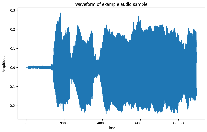
Let’s now visualize the waveform.
audio = estd.MonoLoader(
    filename=os.path.join("..", "audio", "testing_samples", "test_1.wav")
)()

plt.figure(figsize=(10, 6))
plt.plot(audio)
plt.title("Waveform of example audio sample")
plt.xlabel("Time")
plt.ylabel("Amplitude")
plt.show()
Representing audio in the frequency domain#
You might have heard about the Fourier transform. In a few words, it is basically a transformation in which a signal represented in the time domain is decomposed in the frequency components that are present in the signal. To understand that statement, it is important to note that an audio signal is formed by the combination of multiple sinusoids, which are oscillatory signals defined by the following formula:
In other words, each sinusoid is defined by a particular amplitude \(A\), frequency \(f\), and phase \(\phi\), and follows a sinusoidal behaviour, oscillating at the given frequency. The variable \(t\) represents the time vector, in which we are capturing or analyzing the signal. Let’s generate a sinusoid at frequency 440Hz.
Important
Be careful with the volume (btw given by the amplitude \(A\)) when listening to single sinusoids (aka pure tones). It might be harmful, specially if listened with headphones and for a long time.
t = np.arange(0, 1, 1/44100)  # Duration: 1s, sampling rate: 44100Hz
sinusoid_440 = np.sin(2*np.pi*440*t + 0)

# Playing sinusoid of 440Hz
ipd.Audio(sinusoid_440, rate=44100)
The Fourier’s Theorem basically states that any signal can be decomposed into an overlap of several of these sinusoids. Why is that relevant?. Let’s take a look at some different sinusoids.
sinusoid_220 = np.sin(2*np.pi*220*t + 0)

# Playing sinusoid of 220Hz
ipd.Audio(sinusoid_220, rate=44100)
sinusoid_880 = np.sin(2*np.pi*880*t + 0)

# Playing sinusoid of 880Hz
ipd.Audio(sinusoid_880, rate=44100)
Higher frequencies are high pitched, while lower frequencies sound lower in our ears. In practice, computing the frequencies that are present in a music signal provides a lot of relevant information to understand the signals and their content. Depending on the type of sound, the timbre, the notes played in case the source is a musical instrument, the frequency representation of the signal will look several various different ways.
Within the context of computational analysis of a musical repertoire, the frequency domain is useful for many purposes, e. g. to understand the timbre of particular instruments, to capture the notes or melodies that are being performed, and many more. In a ML/DL scenario, frequency-based representations of audio signals are broadly used as input feature for models, providing notable advantages for many tasks. That is why, several approaches within the field of ASP and MIR build on top of this representation, which in many cases captures more information that the raw waveform.
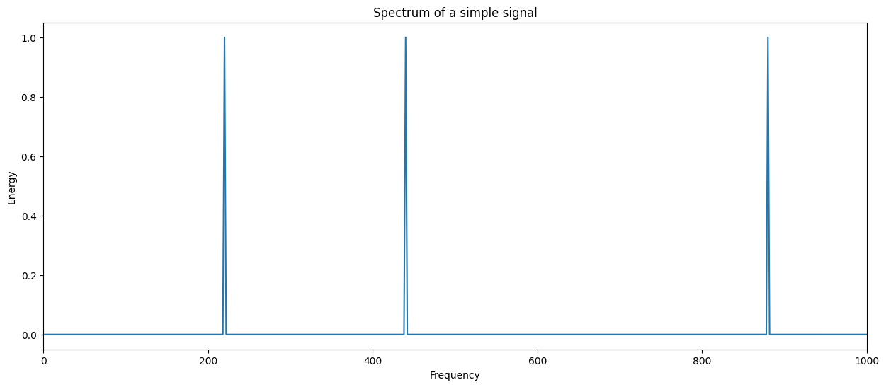
Let’s now visualise, in practise, how a Fourier transform, also known as spectrum of a particular signal looks like:
# We sum the three sinusoids
signal = np.array(
    sinusoid_220 + sinusoid_440 + sinusoid_880,
    dtype=np.single,
)

# We create the spectrum of the signal
spectrum = estd.Spectrum()
window = estd.Windowing(type="hann")
signal_spectrum = spectrum(window(signal))

# We create a x vector to represent the frequencies
xf = np.arange(0, len(signal_spectrum), 1)

plt.figure(figsize=(15, 6))
plt.plot(xf, signal_spectrum)
plt.xlabel("Frequency")
plt.ylabel("Energy")
plt.xlim(0, 1000)  # Limiting view to area of interest
plt.title("Spectrum of a simple signal")
plt.show()
Note
We could also use estd.FFT(), with FFT standing for (Fast Fourier Transform). However, this function does not disregard the complex part generated by the transformation. For more information see the documentation.
Note that the peaks are showing up exactly where the frequencies of the considered sinusoids are. Let us remark at this point an important implication of the sampling frequency here. Given the Nyquist-Shannon theorem, we can just correctly represent the frequency values \(f\) if \(f <= f_s / 2\), being \(f_s\) the sampling frequency of the signal. Therefore, the higher the \(f_s\), the more detail we do have in time, but also the wider the frequency range we can evaluate.
Going back to the spectrum we have plotted above, note that this representation is OK for this use case, however, trying to compute the spectrum for a complete Carnatic or Hindustani music recording will not be very useful, since a massive amount of different sinusoids will appear in an entire performance. For that reason, in a computational musicology scenario, we need a representation that also considers the time dimension.
Time-frequency representation#
A spectrogram, commonly computed using the STFT (Short-Time Fourier Transform), is a time-frequency representation in which a chain of spectrums are calculated from a signal by sliding, with a particular hop size a window of particular window size (or frame size) which indicates the time section in which to apply the frequency decomposition. We always use window size > hop size, therefore there is an overlap of windows, which actually provides a smoother chaining and better frequency analysis. A particular window function is applied to each frame to ensure a more natural overlap. For our computational musicology studies, this representation is very important.
We will use librosa in this case: a Python-based package for audio signal processing. librosa includes nice visualisation tools. Let us show how a time-frequency representation looks like, and how we can compute it in a few steps.
import librosa
import librosa.display
# Computing time-frequency representation for signal above
D = librosa.stft(signal)  # STFT of y
S_db = librosa.amplitude_to_db(np.abs(D), ref=np.max)

# And plotting!
fig, ax = plt.subplots(figsize=(15, 6))
img = librosa.display.specshow(S_db, x_axis='time', y_axis='linear', ax=ax)
ax.set(title='Time-frequency representation')
ax.set(ylim=[0, 2000])
fig.colorbar(img, ax=ax, format="%+2.f dB");
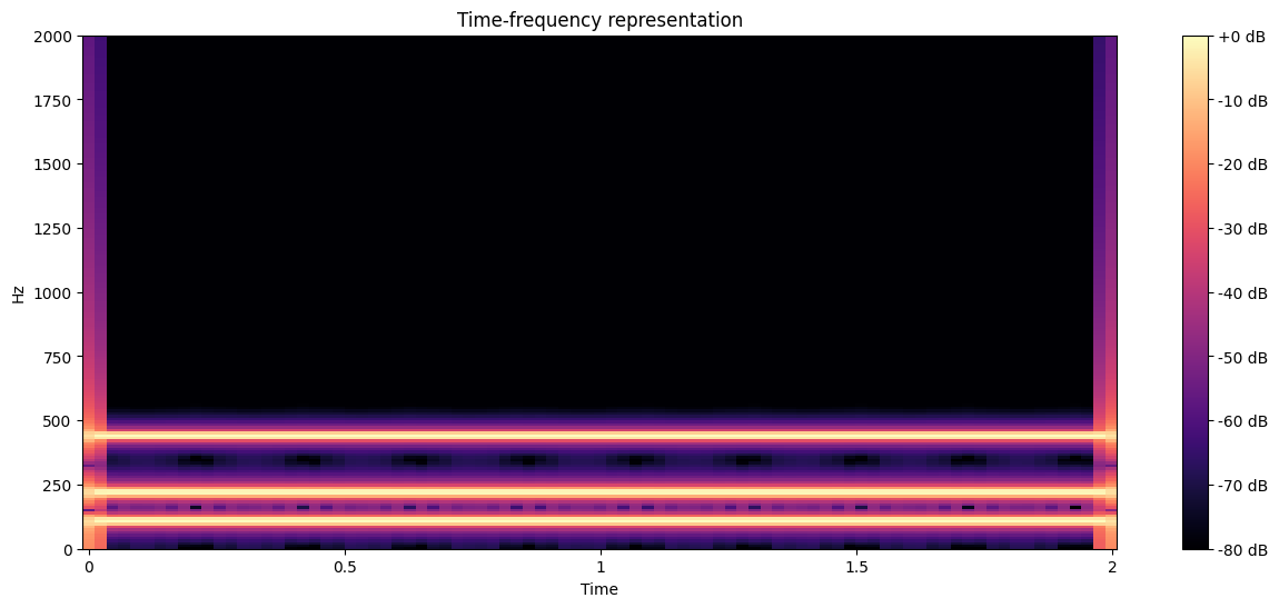
Let’s now plot a more applied signal. We will use a testing audio of 2 seconds, and observe how it looks like.
# librosa may also be used to load audio
y, sr = librosa.load(
    os.path.join("..", "audio", "testing_samples", "test_1.wav")
)

# Computing time-frequency representation for signal above
D = librosa.stft(y)  # STFT of y
S_db = librosa.amplitude_to_db(np.abs(D), ref=np.max)

# And plotting!
fig, ax = plt.subplots(figsize=(15, 6))
img = librosa.display.specshow(S_db, x_axis='time', y_axis='linear', ax=ax)
ax.set(title='Time-frequency representation')
ax.set(ylim=[0, 2000])
fig.colorbar(img, ax=ax, format="%+2.f dB");
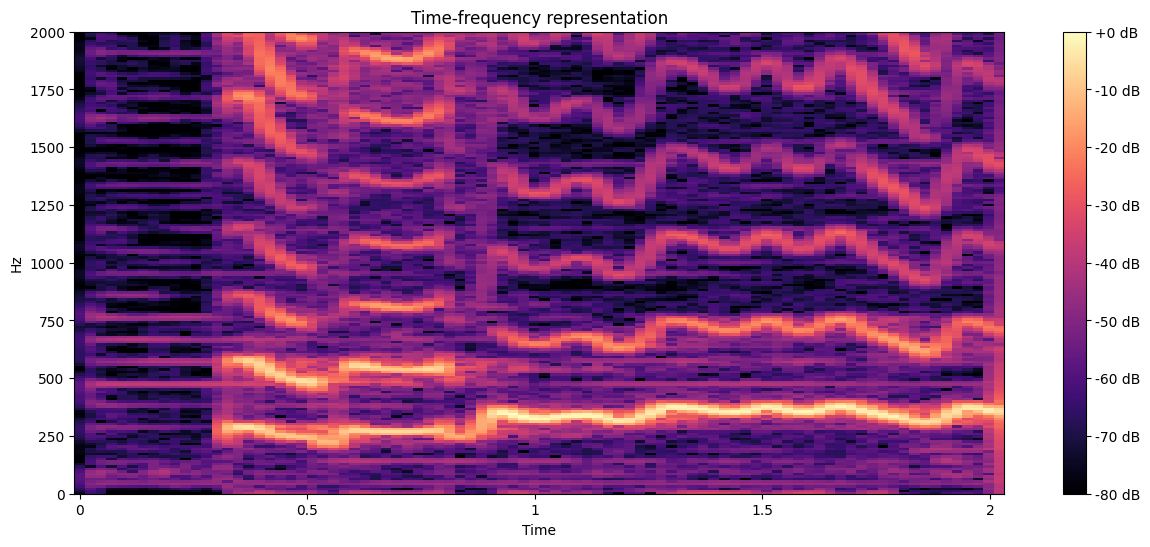
We see that, since multiple pitches are being sung (even in only two seconds), this representation is more appropiate to use. We will refer to the time-frequency representation (aka spectrogram) many times durinng the tutorial, so make sure to understand it clearly.
Other variants may be computed from the spectrogram, e.g. mel-spectrogram. Also, other time-frequency representations more specific for particular tasks may be used, e.g. chroma features. No explicit use of these is included in this tutorial, but we suggest the reader to go through them. These are very important in the field of ASP and MIR.