Meter analysis

In the musical introduction, the main rhythmic characteristics of Carnatic and Hindustani traditions are provided. The presented hierarchical form of a tala is targeted in [SS14b], using a supervised approach on top of spectral hand-crafted features that capture tempo and onsets in the signal. Bayesian models are found to be the most capable of capture the rhythmic cycles in music signals, first applied in the form of particle filters [SHCS15] for an efficient inference, showing competetitive results on Carnatic recordings. The said approach is futher extended to a generalized model to capture long cycles [SHTCS16], being this very convenient for rhythm tracking in Hindustani Music.

## Installing (if not) and importing compiam to the project
import importlib.util
if importlib.util.find_spec('compiam') is None:
    ## Bear in mind this will only run in a jupyter notebook / Collab session
    %pip install git+git://github.com/MTG/compIAM.git
import compiam

# Import extras and supress warnings to keep the tutorial clean
import os
from pprint import pprint
import IPython.display as ipd

import warnings
warnings.filterwarnings('ignore')

Carnatic and Hindustani Music Rhyhtm datasets

That is a precise moment to introduce the (CompMusic) Carnatic and Hindustani Rhythm Datasets. These datasets, which include audio recordings, musically-relevant metadata, and beat and meter annotations, can be downloaded from Zenodo under request and used through the mirdata dataloaders available from release 0.3.7. These dataset present useful for the metrical and beat estimation research on Indian Art Music.

Let’s initialise an instance of these datasets and browse through the available data.

cmr = compiam.load_dataset(
    "compmusic_carnatic_rhythm",
    data_home=os.path.join("../audio/mir_datasets"),
    version="full_dataset"
)
cmr

The compmusic_carnatic_rhythm dataset
----------------------------------------------------------------------------------------------------


Call the .cite method for bibtex citations.
----------------------------------------------------------------------------------------------------


CompMusic Carnatic Music Rhythm class

    Args:
        track_id (str): track id of the track
        data_home (str): Local path where the dataset is stored. default=None
            If `None`, looks for the data in the default directory, `~/mir_datasets`

    Attributes:
        audio_path (str): path to audio file
        beats_path (srt): path to beats file
        meter_path (srt): path to meter file

    Cached Properties:
        beats (BeatData): beats annotation
        meter (string): meter annotation
        mbid (string): MusicBrainz ID
        name (string): name of the recording in the dataset
        artist (string): artists name
        release (string): release name
        lead_instrument_code (string): code for the load instrument
        taala (string): taala annotation
        raaga (string): raaga annotation
        num_of_beats (int): number of beats in annotation
        num_of_samas (int): number of samas in annotation

    ----------------------------------------------------------------------------------------------------

For showcasing purposes, we include a single-track version of the (CompMusic) Carnatic Rhythm Dataset within the materials of this tutorial. This dataset is private, but can be requested and downloaded for research purposes.

Reading through the dataset details we observe the available data for the tracks in the dataloader. We will load the tracks and select the specific track we have selected for tutoring purposes. Bear in mind that you can access the list of identifiers in the dataloader with the .track_ids attribute.

track = cmr.load_tracks()["10001"]

Let’s print out the available annotations for this example track.

track.beats

BeatData(confidence, confidence_unit, position_unit, positions, time_unit, times)

BeatData is an annotation type that is used in mirata to store information related to rhythmic beats. We will print the time-steps for the first 20 annotated beats.

track.beats.times[:20]

array([ 0.627846,  1.443197,  2.184898,  2.944127,  3.732721,  4.476644,
        5.293333,  6.078821,  6.825918,  7.639819,  8.42873 ,  9.201905,
       10.168209, 10.982404, 11.784082, 12.55551 , 13.325556, 14.09551 ,
       14.858866, 15.585941])

Let’s also observe the actual magnitude of these annotations.

track.beats.time_unit

's'

We have confirmed that the beats are annotated in s, seconds. We can also observe the positons in the cycle (if available) that each of the beats occupy.

track.beats.positions[:20]

array([1, 2, 3, 4, 5, 6, 7, 8, 1, 2, 3, 4, 5, 6, 7, 8, 1, 2, 3, 4])

mirdata annotations have been created aiming at providing standardized and useful data structures for MIR-related annotations. In this example we showcase the use of BeatData, but many more annotation types are included in mirdata. Make sure to check them out!.

Let’s now observe how the meter annotations looks like.

track.meter

'8/4'

Unfortunately, no tools to track the beats or the meter in Indian Art Music performances are available in compiam as of now. We are looking forward to covering these tasks in the near future!

Nonetheless, in this section we would like to showcase a relevant tool to track the aksharas in a music recording.

Akshara pulse tracker

Let’s first listen to the audio example we are going to be using to showcase this tool. We will just load the first 30 seconds (we can just slice the audio array from 0 to \(f_{s} * sec\), being \(sec\) the integer number of seconds to get).

# Let's listen to 30 seconds of the input audio
track = cmr.load_tracks()["10001"]
audio, sr = track.audio
ipd.Audio(
    data=audio[:, :10*sr],
    rate=sr
)

We now import the onset detection tool from compiam.rhythm.meter.

# We import the tool
from compiam.rhythm.meter import AksharaPulseTracker

# Let's initialize an instance of the tool
apt = AksharaPulseTracker()

Likewise the other extractors and models in compiam (if not indicated otherwise), the method for inference takes an audio path as input.

predicted_aksharas = apt.extract(track.audio_path)

Let’s see all the information about the aksharas that the system estimates.

list(predicted_aksharas.keys())

['sections', 'aksharaPeriod', 'aksharaPulses', 'APcurve']

Let’s now print out some details on each estimated aspect of the aksharas.

predicted_aksharas['sections']

{'startTime': [0.0], 'endTime': [148.979], 'label': 'Kriti'}

predicted_aksharas['aksharaPeriod']

0.191

predicted_aksharas['aksharaPulses'][:4]

[1.0247879048950763, 1.2306540519864908, 1.312782895250968, 1.4763296264147416]

predicted_aksharas['APcurve'][:4]

[[0.0, 0.1895734597156398],
 [0.4992290249433111, 0.1895734597156398],
 [0.9984580498866213, 0.1895734597156398],
 [1.4976870748299325, 0.1895734597156398]]

We can now use the compiam.visualisation to plot the input audio with the annotations on top.

from compiam.visualisation.audio import plot_waveform
help(plot_waveform)

Help on function plot_waveform in module compiam.visualisation.audio:

plot_waveform(input_data, t1, t2, labels=None, input_sr=44100, sr=44100, output_path=None, verbose=False)
    Plotting waveform between two given points with optional labels
    
    :param input_data: path to audio file or numpy array like audio signal
    :param input_sr: sampling rate of the input array of data (if any). This variable is only
        relevant if the input is an array of data instead of a filepath.
    :param t1: starting point for plotting
    :param t2: ending point for plotting
    :param labels: dictionary {time_stamp:label} to plot on top of waveform
    :param sr: sampling rate
    :param output_path: optional path (finished with .png) where the plot is saved

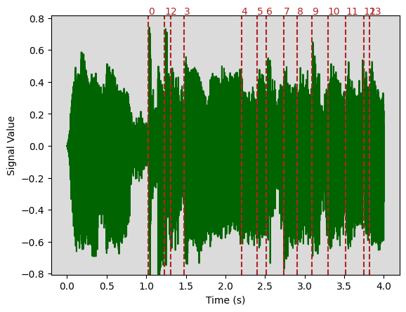
We observe that the labels input variable in plot_waveforms needs to be a dict with the following format: {time-step: label}, while our estimation is basically a list of pulses. Therefore, we first need to convert the prediction into a dictionary. We take the predicted beats, convert these into a dictionary, and plot them on top of the waveform of the input signal again, in order to compare between the estimation and the ground-truth above.

pulses = predicted_aksharas['aksharaPulses']
predicted_beats_dict = {
    time_step: idx for idx, time_step in enumerate(pulses)
}

# And we plot!
plot_waveform(
    input_data=track.audio_path,
    t1=0,
    t2=4,
    labels=predicted_beats_dict,
);

<Figure size 2000x500 with 0 Axes>