Exploring Carnatic Performance

Thomas Nuttall, Genís Plaja-Roglans, Lara Pearson, Brindha Manickavasakan, Xavier Serra.

This notebook serves to demonstrate the wide range of tools available as part of the compIAM package. We demonstrate their use on a single performance from the Saraga Audiovisual Dataset, the multi-modal portion of the wider Saraga Dataset [SGRS20]. The tools showcased here are not accompanied by exhaustive usage documentation, which can be found in their respective pages in other parts of this webbook, links for which are provided in each section.

Contents

1. Import Dependencies and Data

2. Loading and Visualising Data

   • Multitrack Player

   • Video and Gesture Tracks

3. Feature Extraction

   • Tonic Identificaton

   • Raga Recognition

   • Music Source Separation

   • Pitch Extraction

   • Percussion Onset Detection

   • Melodic Pattern Detection

1. Import Dependencies and Data

Due to restrictions in accessing the Saraga API through the Github hosted webbook, we access the data through a custom shared Google drive created specifically for this tutorial. Users wishing to work with audio from Saraga should follow the instructions here.

## Installing (if not) and importing compiam to the project
import importlib.util
%pip install -U compiam==0.4.1  # Install latest version of compiam
%pip install essentia
%pip install "torch==1.13"
%pip install "tensorflow==2.15.0" "keras<3"

import compiam
import essentia.standard as estd

# Import extras and supress warnings to keep the tutorial clean
import os
import shutil
import gdown
import zipfile

import numpy as np
import IPython.display as ipd
import matplotlib.pyplot as plt

from pprint import pprint

import warnings
warnings.filterwarnings('ignore')

AUDIO_PATH = os.path.join("..", "audio", "demos")

NOTE: If working on Collab, please uncomment and run this cell below, otherwise, don’t!

#AUDIO_PATH = "./"  ## Run if working on collab!

Since Saraga Audiovisual is a fresh new dataset very recently published in ISMIR 2024 (San Francisco, USA), it is still not available through mirdata and compIAM. However, we will manually download and load an example concert recording from this dataset, a concert performed by Dr. Brindha Manickavasakan during the December Season in Chennai in 2023. Dr. Manickavasakan is also a collaborator of the ongoing efforts on the computational melodic analysis of Carnatic Music in a collaboration between a group of researchers from the Music Technology Group and Dr. Lara Pearson from the Max Plank Institute of Empirical Aesthetics.

url = "https://drive.google.com/uc?id=1iR0bfxDLQbH8fEeHU_GFsg2kh7brZ0HZ&export=download"
output =  os.path.join(AUDIO_PATH,  "dr-brindha-manickavasakan.zip")
gdown.download(url, output, quiet=False)

# Unzip file
with zipfile.ZipFile(output, 'r') as zip_ref:
    zip_ref.extractall(AUDIO_PATH)

# Delete zip file after extraction
os.remove(output)

Alright, the data is downloaded and uncompressed. Let’s get the path to it and analyse a rendition from the concert.

2. Loading and visualising the data

We work with a single performance from a concert by Brindha Manickavasakan at the Arkay Convention Center, recorded in 2023 in Chennai, South India. The composition is Bhavanuta by Tyaagaraaja in raga mohanam.

rendition = "Bhavanuta"
folder_path = os.path.join(AUDIO_PATH, 'dr-brindha-manickavasakan', rendition)

For 100s of performances in the Saraga dataset, the audio stems corresponding to each instrument/perfromer are available. In this performance, this constitutes the lead vocal, the mridangam (left and right microphone), the violin, and the tanpura. The full mix of all instruments is also available.

Let us select the preview versions of the multitrack audio, which are shortened and compressed versions of the rendition for easier handling of the previsualisation.

audio_path_pre = os.path.join(folder_path, "preview", f"{rendition}.mp3")
mrid_left_path_pre = os.path.join(folder_path, "preview", f"{rendition}.mridangam-left.mp3")
mrid_right_path_pre = os.path.join(folder_path, "preview", f"{rendition}.mridangam-right.mp3")
violin_path_pre = os.path.join(folder_path, "preview", f"{rendition}.multitrack-violin.mp3")
vocal_path_pre = os.path.join(folder_path, "preview", f"{rendition}.multitrack-vocal.mp3")
tanpura_path_pre = os.path.join(folder_path, "preview", f"{rendition}.tanpura.mp3")

1.1 Multitrack player

We can use the compIAM waveform player to visualise and listen to all of the tracks at the same time, panning, or changing the volume of each as required.

from compiam.visualisation.waveform_player import Player

# list of paths to load and listen
all_audio_paths = [
    vocal_path_pre,
    violin_path_pre,
    mrid_left_path_pre,
    mrid_right_path_pre,
    tanpura_path_pre
]
# List of labels for each path
all_names = ["Vocal", "Violin", "Mridangam left", "Mridangam right", "Tanpura"]

Player(all_names, all_audio_paths)

/opt/hostedtoolcache/Python/3.11.11/x64/lib/python3.11/site-packages/compiam/visualisation/waveform_player/waveform-playlist/
multi-channel.html

1.2 Video and Gesture Tracks

The Saraga Audiovisual dataset includes videos of the performances and gesture tracks extracted using MMPose for the lead performer. Let’s take a look at a sample for this performance.

import cv2
import IPython.display as ipd
from IPython.core.display import HTML

vid_out_path =  f'{folder_path}/output_segment.mp4'

# Load keypoints and scores
keypoints_file = f"{folder_path}/singer/Brindha_Manickavasakan_Segment1_0-513_kpts.npy"
scores_file = f"{folder_path}/singer/Brindha_Manickavasakan_Segment1_0-513_scores.npy"
video_file = f"{folder_path}/{rendition}.mov"  # Replace with your video file

keypoints = np.load(keypoints_file)
scores = np.load(scores_file)

# Skeleton for 135 keypoints
# Skeleton for 135 keypoints (MMPose)
skeleton = [
    (0, 1), (1, 2),  # Eyes (left to right)
    (0, 3), (0, 4),  # Nose to ears (left and right)
    (5, 6),          # Shoulders (left and right)
    (5, 7), (7, 9),  # Left arm (shoulder -> elbow -> wrist)
    (6, 8), (8, 10),
    (11,12),  # Right arm (shoulder -> elbow -> wrist)
    (5, 11), (6, 12), # Shoulders to hips
    (11, 13), (13, 15), # Left leg (hip -> knee -> ankle)
    (12, 14), (14, 16)  # Right leg (hip -> knee -> ankle)
]

# Open video file
cap = cv2.VideoCapture(video_file)
fps = int(cap.get(cv2.CAP_PROP_FPS))  # Frames per second
frame_width = int(cap.get(cv2.CAP_PROP_FRAME_WIDTH))
frame_height = int(cap.get(cv2.CAP_PROP_FRAME_HEIGHT))

# Define start and end frames for the 20-second segment
start_time = 10  # Start time in seconds (adjust as needed)
end_time = start_time + 20  # End time in seconds
start_frame = int(start_time * fps)
end_frame = int(end_time * fps)

# Output video writer
out = cv2.VideoWriter(vid_out_path, cv2.VideoWriter_fourcc(*'mp4v'), fps, (frame_width, frame_height))

# Process the selected frames
frame_idx = 0
while cap.isOpened():
    ret, frame = cap.read()
    if not ret:
        break

    if start_frame <= frame_idx < end_frame:
        # Get keypoints and scores for the current frame
        if frame_idx < len(keypoints):
            frame_keypoints = keypoints[frame_idx]
            frame_scores = scores[frame_idx]

            # Draw keypoints and skeleton
            for i, (x, y) in enumerate(frame_keypoints):
                # Only draw if confidence score is above threshold
                if frame_scores[i] > 0.5:  # Adjust threshold as needed
                    cv2.circle(frame, (int(x), int(y)), 5, (0, 255, 0), -1)

            # Draw skeleton
            for connection in skeleton:
                start, end = connection
                if frame_scores[start] > 0.5 and frame_scores[end] > 0.5:
                    x1, y1 = frame_keypoints[start]
                    x2, y2 = frame_keypoints[end]
                    cv2.line(frame, (int(x1), int(y1)), (int(x2), int(y2)), (255, 0, 0), 2)

        # Write frame to output video
        out.write(frame)

    frame_idx += 1

    # Stop processing after the end frame
    if frame_idx >= end_frame:
        break

# Release resources
cap.release()
out.release()
cv2.destroyAllWindows()
print("20-second video segment processing complete. Output saved as 'output_segment.mp4'")

20-second video segment processing complete. Output saved as 'output_segment.mp4'

import subprocess
subprocess.run(["ffmpeg", "-vcodec", "libx264",  "-acodec", "aac", f"{vid_out_path.replace('.mp4', '_re-encoded.mp4')}"])

ffmpeg version 6.1.1-3ubuntu5 Copyright (c) 2000-2023 the FFmpeg developers
  built with gcc 13 (Ubuntu 13.2.0-23ubuntu3)
  configuration: --prefix=/usr --extra-version=3ubuntu5 --toolchain=hardened --libdir=/usr/lib/x86_64-linux-gnu --incdir=/usr/include/x86_64-linux-gnu --arch=amd64 --enable-gpl --disable-stripping --disable-omx --enable-gnutls --enable-libaom --enable-libass --enable-libbs2b --enable-libcaca --enable-libcdio --enable-libcodec2 --enable-libdav1d --enable-libflite --enable-libfontconfig --enable-libfreetype --enable-libfribidi --enable-libglslang --enable-libgme --enable-libgsm --enable-libharfbuzz --enable-libmp3lame --enable-libmysofa --enable-libopenjpeg --enable-libopenmpt --enable-libopus --enable-librubberband --enable-libshine --enable-libsnappy --enable-libsoxr --enable-libspeex --enable-libtheora --enable-libtwolame --enable-libvidstab --enable-libvorbis --enable-libvpx --enable-libwebp --enable-libx265 --enable-libxml2 --enable-libxvid --enable-libzimg --enable-openal --enable-opencl --enable-opengl --disable-sndio --enable-libvpl --disable-libmfx --enable-libdc1394 --enable-libdrm --enable-libiec61883 --enable-chromaprint --enable-frei0r --enable-ladspa --enable-libbluray --enable-libjack --enable-libpulse --enable-librabbitmq --enable-librist --enable-libsrt --enable-libssh --enable-libsvtav1 --enable-libx264 --enable-libzmq --enable-libzvbi --enable-lv2 --enable-sdl2 --enable-libplacebo --enable-librav1e --enable-pocketsphinx --enable-librsvg --enable-libjxl --enable-shared
  libavutil      58. 29.100 / 58. 29.100
  libavcodec     60. 31.102 / 60. 31.102
  libavformat    60. 16.100 / 60. 16.100
  libavdevice    60.  3.100 / 60.  3.100
  libavfilter     9. 12.100 /  9. 12.100
  libswscale      7.  5.100 /  7.  5.100
  libswresample   4. 12.100 /  4. 12.100
  libpostproc    57.  3.100 / 57.  3.100
Output #0, mp4, to '../audio/demos/dr-brindha-manickavasakan/Bhavanuta/output_segment_re-encoded.mp4':
[out#0/mp4 @ 0x55fd9e050340] Output file does not contain any stream
Error opening output file ../audio/demos/dr-brindha-manickavasakan/Bhavanuta/output_segment_re-encoded.mp4.
Error opening output files: Invalid argument

CompletedProcess(args=['ffmpeg', '-vcodec', 'libx264', '-acodec', 'aac', '../audio/demos/dr-brindha-manickavasakan/Bhavanuta/output_segment_re-encoded.mp4'], returncode=234)

#video_html = f"""
#<video width="640" height="480" controls>
#  <source src="{vid_out_path}" type="video/mp4">
#  Your browser does not support the video tag.
#</video>
#"""
#ipd.display(HTML(video_html))

from IPython.core.display import Video

Video(vid_out_path.replace('.mp4', '_re-encoded.mp4'), embed=True)

3. Feature Extraction

In this section we extract various audio and musical features from the raw performance audio; the singer tonic, raga, predominant pitch track of the lead vocal melody, source separated vocal audio, downbeat, and repeated melodic patterns.

Let’s first get the path of the full and uncompressed mixture and vocal tracks.

audio_path = os.path.join(folder_path, f"{rendition}.wav")
vocal_path = os.path.join(folder_path, f"{rendition}.multitrack-vocal.wav")

2.1 Tonic Identification

The tonic of the lead singer is useful for normalising pitch and comparing with other performers. Here we can use the TonicIndianMultiPitch tool which is available through Essentia and compIAM.

# Importing the tool
from compiam.melody.tonic_identification import TonicIndianMultiPitch

# We first initialize the tool we have just imported
tonic_multipitch = TonicIndianMultiPitch()

tonic = tonic_multipitch.extract(audio_path)

print(f'Performer tonic: {round(tonic, 2)} Hz')

Performer tonic: 196.42 Hz

We can quickly listed to the estimated tonic on top of the original audio to perceptually evaluate if the tonic sounds reasonable to the chosen rendition.

# Let's get the audio for the track
sr = 44100
audio_mix = estd.MonoLoader(filename=audio_path, sampleRate=sr)()

# Let's synthesize a tambura
synthesized_tambura = 0.75*np.sin(
    2*np.pi*float(tonic)*np.arange(0, len(audio_mix)//sr, 1/sr)
)
# Adding some harmonics
synthesized_tambura += 0.25*np.sin(
    2*np.pi*float(tonic)*2*np.arange(0, len(audio_mix)//sr, 1/sr)
)
synthesized_tambura += 0.5*np.sin(
    2*np.pi*float(tonic)*3*np.arange(0, len(audio_mix)//sr, 1/sr)
)
synthesized_tambura += 0.125*np.sin(
    2*np.pi*float(tonic)*4*np.arange(0, len(audio_mix)//sr, 1/sr)
)

# We take just a minute of music (60 seg * 44100)
audio_tonic = audio_mix[:60*sr] + synthesized_tambura[:60*sr]*0.02

# And we play it!
ipd.Audio(
    data=audio_tonic[None],
    rate=sr,
)

That sounds good! This is the tonic of the recording. This is a really valuable information that allows us to characterise and normalize the melodies, and may give relevant information about the artist and performed concert.

For further reference, please visit the tonic identification page.

2.2 Raga Recognition

Whilst raga metadata is available as part of Saraga, compIAM contains a raga identifier, DeepSRGM. We can automatically identifier the raga using this tool. Be aware, this model was trained on the ragas; Bhairav, Madhukauns, Mōhanaṁ, Hamsadhvāni, Varāḷi, Dēś, Kamās, Yaman kalyāṇ, and Bilahari, Ahira bhairav, only and hence can only assign those classes.

from compiam import load_model

# This model uses tensorflow in the backend!
deepsrgm = load_model("melody:deepsrgm")

# Computing features
feat = deepsrgm.get_features(vocal_path)

# Predict raga using subset of features for faster prediction
predicted_raga = deepsrgm.predict(feat[:10])
print(f'Raga: {predicted_raga}')

2.3 Music Source Separation

Music source separation is the task of automatically estimating the individual elements in a musical mixture. Apart from its creative uses, it may be very important as builing block in research pipeline, acting as a very handy pre-processing step [PRMSS23]. To carefully analyse the singing voice and its components, normally having it isolated from the rest of the instruments is beneficial.

There are several models in the literature to address this problem, most of them based on deep learning architectures, some of them provide pre-trained weights such as Demucs [DUBB19] or Spleeter [HKVM20], the latter is broadly used in Carnatic Music computational research works. However, thes systems have two problems: (1) the training data of these models does normally not include Carnatic Music examples, therefore there are instruments and practices which are completely unseed by these models, and (2) these models have a restricted set of target elements, namely (vocals, bass, drums, and other), which does not fit to Carnatic Music arrangements at all.

To address problem (1), there have been few attemps on trying to use the multi-stem data presented above to develop Carnatic-tailored source separation systmes, although the available multi-stem recordings are collected from mixing consoles in live performances, and therefore the individual tracks are noisy (have background leakage from the rest of the sources). We can test one example of these systems here: {cite}``.

# Make sure proper TF version is installed
%pip install "tensorflow==2.15.0" "keras<3"

from compiam import load_model

# This model uses tensorflow in the backend!
separation_model = load_model("separation:cold-diff-sep")
SEPARATION_SR = separation_model.sample_rate

audio_mix = estd.MonoLoader(filename=audio_path, sampleRate=SEPARATION_SR)()
separation_input = audio_mix[SEPARATION_SR*60:SEPARATION_SR*90]
separated_vocals = separation_model.separate(
    separation_input,
    input_sr=SEPARATION_SR
)

ipd.Audio(separated_vocals, rate=SEPARATION_SR)

Let’s try to be a bit more restrictive using the configuration of the separation algorithm.

audio_mix = estd.MonoLoader(filename=audio_path, sampleRate=SEPARATION_SR)()
separation_input = audio_mix[SEPARATION_SR*60:SEPARATION_SR*90]
separated_vocals = separation_model.separate(
    separation_input,
    input_sr=SEPARATION_SR,
    clusters=8,
    scheduler=7,
)

ipd.Audio(separated_vocals, rate=SEPARATION_SR)

Although there is still a long way to go on this problem, the ongoing efforts on improving on the separation of singing voice (and also the rest of the instrumentation!) for Carnatic Music set an interesting baseline to bulid on top of.

For further reference, please visit the music source separation page.

2.4 Pitch Extraction

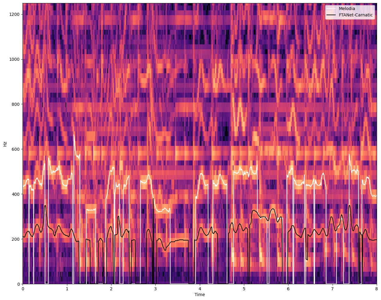
The f0 pitch track of the predominant vocal melody has proved useful for range of computational analysis tasks in Indian Art Music. We can extract this for our performance using Melodia [SG12], a broadly used knowledge-based method. We will also test a recently published DL model to achieve the same goal: FTA-Net model, which has been trained specifically for the Carnatic Music use case and included in compIAM as well [PRNP+23].

# Make sure proper TF version is installed
%pip install "tensorflow==2.15.0" "keras<3"

from compiam import load_model
from compiam.melody.pitch_extraction import Melodia

melodia = Melodia() 
ftanet_carnatic = load_model("melody:ftanet-carnatic")
PITCH_EXTRACTION_SR = 44100

To extract an example pitch track, we first load 30s of the mixture recording, and run prediction with both methods. Once the methods are initialized, running pitch extraction is easily done in one line of code.

import librosa
import librosa.display
import numpy as np
import matplotlib.pyplot as plt

audio_mix = estd.MonoLoader(filename=audio_path, sampleRate=PITCH_EXTRACTION_SR)()
prediction_input = audio_mix[PITCH_EXTRACTION_SR*60:PITCH_EXTRACTION_SR*90]

# Predominant extraction models
melodia_pitch_track = melodia.extract(prediction_input, input_sr=PITCH_EXTRACTION_SR)
ftanet_pitch_track = ftanet_carnatic.predict(prediction_input, input_sr=PITCH_EXTRACTION_SR)

Let’s now plot both pitch tracks and compare!

fig, ax = plt.subplots(nrows=1, ncols=1, sharex=True, figsize=(15, 12))
D = librosa.amplitude_to_db(np.abs(librosa.stft(prediction_input)), ref=np.max)
img = librosa.display.specshow(D, y_axis='linear', x_axis='time', sr=PITCH_EXTRACTION_SR, ax=ax);
ax.set_ylim(0, 1250)
ax.set_xlim(0, 8)  # Visualising 8 seconds
plt.plot(
    melodia_pitch_track[:, 0], melodia_pitch_track[:, 1],
    color="white", label="Melodia",
)
plt.plot(
    ftanet_pitch_track[:, 0], ftanet_pitch_track[:, 1],
    color="black", label="FTANet-Carnatic",
)
plt.legend()

<matplotlib.legend.Legend at 0x7f7b5d84d810>

ipd.Audio(prediction_input[:8*PITCH_EXTRACTION_SR], rate=PITCH_EXTRACTION_SR)

See that the violin is fooling the Melodia algorithm which is getting all vocal pitch values one octave above, while FTA-Net is able to get the right pitch values. This is a very common issue when analysing melody in the context of Carnatic Music: the presence of violin shadowing the singing voice is an enormous challenge for the vocal models and algorithms.

Let’s now extract the entire pitch track from the available vocal stem.

pitch_track = ftanet_carnatic.predict(vocal_path, input_sr=PITCH_EXTRACTION_SR)
pitch = pitch_track[:, 1]  # Pitch in Hz
time  = pitch_track[:, 0]  # Time in seconds
timestep  = time[2] - time[1]  # Time in seconds between elements of pitch track

We interpolate small gaps owing to glottal stops or consonant sounds.

from compiam.utils.pitch import interpolate_below_length

pitch = interpolate_below_length(
    pitch,  # track to interpolate
    0,  # value to interpolate 
    200*0.001/timestep  # maximum gap in number sequence elements to interpolate for
)

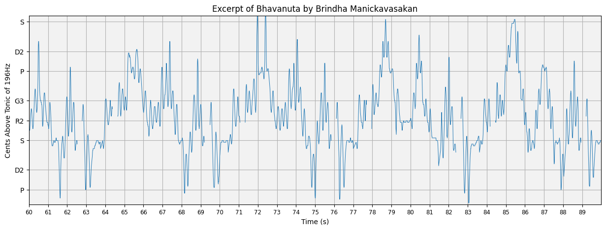
Let’s visualise our pitch plot using the plot_pitch function from compIAM.visualisation.pitch. We can manually change the yticks to correspond to theoretical svara positions by passing a custom dictionary of {ytick labels : y values}. Since we know the raga (from section 2.2) and the singer tonic (from section 2.1). We can use get_svara_pitch_carnatic to query for the svaras relevant to that raga, and pass that dictionary and the tonic to plot_pitch to alter the pitch plot.

from compiam.visualisation.pitch import plot_pitch, flush_matplotlib
from compiam.utils import ipy_audio
from compiam.utils import get_svara_pitch_carnatic

# let's load the audio also
audio = estd.MonoLoader(filename=audio_path, sampleRate=PITCH_EXTRACTION_SR)()

t1 = 60  # in seconds
t2 = 90  # in seconds
t1s = round(t1/timestep)  # in sequence elements
t2s = round(t2/timestep)  # in sequence elements

this_pitch = pitch[t1s:t2s]
this_time = time[t1s:t2s]

silence_mask = this_pitch == 0

svara_pitch = get_svara_pitch_carnatic('mohanam', tonic=tonic)

plot_pitch(
    this_pitch,
    this_time,
    mask=silence_mask,
    yticks_dict=svara_pitch,
    tonic=tonic,
    cents=True,
    title=f'Excerpt of {rendition} by Brindha Manickavasakan'
)

(<Figure size 1500x500 with 1 Axes>,
 <Axes: title={'center': 'Excerpt of Bhavanuta by Brindha Manickavasakan'}, xlabel='Time (s)', ylabel='Cents Above Tonic of 196Hz'>)

Let’s generate a sine wave from this pitch track and listen with the accompanying audio.

import numpy as np

def generate_sine_wave(frequencies, time_points, sampling_rate=44100, harmonics=[1.0]):
    """
    Generate a sine wave with harmonics from a time series of fundamental frequencies.

    Parameters:
        frequencies (numpy.ndarray): Array of fundamental frequencies (Hz).
        time_points (numpy.ndarray): Array of corresponding time points (seconds).
        sampling_rate (int): Sampling rate for the sine wave (samples per second).
        harmonics (list of float): Amplitudes of the harmonics relative to the fundamental frequency.
                                   The list index corresponds to the harmonic order (e.g., [1.0, 0.5] for 1st and 2nd harmonics).

    Returns:
        numpy.ndarray: Generated sine wave with harmonics.
    """
    # Ensure inputs are numpy arrays
    frequencies = np.array(frequencies)
    time_points = np.array(time_points)

    # Generate time values for the entire duration based on the sampling rate
    total_duration = time_points[-1]
    t = np.linspace(0, total_duration, int(total_duration * sampling_rate), endpoint=False)
    
    # Interpolate the frequency values for the generated time points
    interpolated_frequencies = np.interp(t, time_points, frequencies)
    
    # Initialize the wave with the fundamental frequency component
    wave = np.zeros_like(t)
    
    for i, amplitude in enumerate(harmonics):
        harmonic_order = i + 1
        harmonic_frequencies = interpolated_frequencies * harmonic_order
        if harmonic_frequencies.max() > sampling_rate / 2:
            break  # Skip harmonics above Nyquist frequency
        phase = np.cumsum(harmonic_frequencies) / sampling_rate
        wave += amplitude * np.sin(2 * np.pi * phase)

    wave = wave / np.max(np.abs(wave))

    return wave

# Synthesize audio
synthesized_audio = generate_sine_wave(pitch, time, sampling_rate=PITCH_EXTRACTION_SR, harmonics=[1,2,3,4,5])

combined = audio + 0.05*synthesized_audio[:len(audio)]

ipy_audio(audio, t1, t2, sr=PITCH_EXTRACTION_SR)

Pitch curves are a really important feature for the computational analysis of Carnatic Music. The important and very much present ornamentation of notes and transitions between notes, it is better represented with continuous pitch value arrays. However, since the lead melodic instruments are normally found mixed with accompanying instruments, we require methods that are able to capture the melodies in the presence of background music.

Pitch curves, or tracks, can be used for a list of tasks that aim at extracting relevant melodic information from the performed melodies. Also, several classification and tagging tasks (e.g. raga classification), build on top of melodic features, normally including pitch information, whether explicitly, or embedded in other representations.

For further reference, please visit the pitch extraction page.

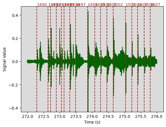
2.5 Percussion onset detection

# We import the tool
from compiam.rhythm.meter import AksharaPulseTracker

# Let's initialize an instance of the tool
apt = AksharaPulseTracker()

predicted_aksharas = apt.extract(audio_path)

from compiam.visualisation.audio import plot_waveform

pulses = predicted_aksharas['aksharaPulses']
predicted_beats_dict = {
    time_step: idx for idx, time_step in enumerate(pulses)
}

# And we plot!
plot_waveform(
    input_data=audio_path,
    t1=272,
    t2=276,
    labels=predicted_beats_dict,
);

<Figure size 2000x500 with 0 Axes>

2.6 Melodic pattern discovery

In this section we demonstrate the task of repeated melodic motif identification in Carnatic Music. The methodologies used are presented in [NPRPS22a] and [PRNP+23] for which compIAM repository serves as the most up to date and well-maintained implementation.

In the compIAM documentation we can see that the tool we showcase in this page has torch as a dependency for the DL models.

To identify repeated melodic patterns in our audio we use melodic features computed for windows across the entirety of the track and use the pairwise similarity between these to identify regions of consistent high-similarity… in theory corresponding to melodic repetitions.

In principle, any set of features can be used in this section. The extent to which these features capture the aspects of melody we care about will define their usefulness for the task.

Here we use melodic features extracted using a Complex Autoencoder (CAE). Mapping signals onto complex basis functions learnt by the CAE results in a magnitude space that has proven to achieve state-of-the-art results in repeared section discovery for audio [LAD19].

The CAE we use here is provided via compiam.load_models and has been trained on the entirety of the Carnatic Saraga dataset for which we have multitrack recordings.

# Pattern Extraction for a Given Audio
from compiam import load_model

# Feature Extraction: CAE features
cae = load_model("melody:cae-carnatic")

Extracting features across the entirety of our chosen audio…

# returns magnitude and phase
ampl, _ = cae.extract_features(audio_path)
ampl

We want to compute the pairwsie self similarity between all combinations of features. With some Carnatic performances lasting up to over an hour, this can often be an expensive computation. There are many regions of the track that we are not interested in (such as silence), or that serve as plausible segmentation points for repeated melodic patterns (such as long periods of stability/silence).

compiam.melody.pattern.self_similarity provides a method of computing the self similarity whilst skipping the computation for regions defined by a user specified exclusion mask.

from compiam.melody.pattern import self_similarity

from compiam.utils.pitch import (
    extract_stability_mask,
    pitch_seq_to_cents,
)

pitch_cents = pitch_seq_to_cents(pitch, tonic=tonic)

First let’s compute the mask corresponding to regions we do not want to compute, these are regions of silence:

silence_mask = pitch==0

And regions of consistent stability. To identify regions of consistent stability we use compiam.utils.pitch.extract_stability_mask. extract_stability_mask computes the average deviation of pitch from the mean in a series of windows across the track. If the deviation exceeds a certain threshold for a sufficient number of consecutive windows, the area is marked as stable (1 in the returned mask), else 0.

stability_mask = extract_stability_mask(
    pitch=pitch_cents,  # pitch track
    min_stab_sec=1.0,  # minimum cummulative length of stable windows to warrant annotation
    hop_sec=0.2,  # hop length in seconds
    var=60,  # minimum variation from the mean in each window to be considered stable
    timestep=timestep  # time in seconds between consecutice elements in <pitch>
)

We can inspect the result to check it has worked correctly

t1 = 330  # in seconds
t2 = t1 + 10  # in seconds

t1s = round(t1/timestep)  # in sequence elements
t2s = round(t2/timestep)  # in sequence elements

this_pitch = pitch[t1s:t2s]
this_time = time[t1s:t2s]
this_silence_mask = silence_mask[t1s:t2s]
this_stable_mask = stability_mask[t1s:t2s]

# Get pitch plot
fig, ax = plot_pitch(
    this_pitch,
    this_time, 
    mask=this_silence_mask,
    tonic=tonic,
    yticks_dict=svara_pitch,
    cents=True,
    title=f'Excerpt of {rendition} by Brindha Manickavasakan'
)

# On alternative axis plot stable mask values
ax2 = ax.twinx()
ax2.plot(this_time, this_stable_mask, 'g', linewidth=1, alpha=1, linestyle='--')
ax2.set_yticks([0,1])
ax2.set_ylabel("Is stable region?")
    
# Accompanying audio
ipy_audio(audio, t1, t2, sr=sr)

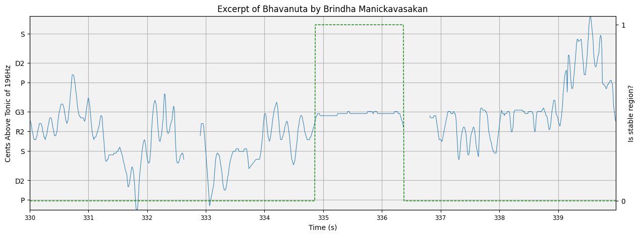
Here the green line is to be read from the right-hand y-axis… is the region stable or not?

Looks good! Let’s combine the two masks:

exclusion_mask = np.logical_or(silence_mask==1, stability_mask==1)

And compute the self similarity self_similarity():

# Mask of regions not interested in cite kaustuv, the papers that use 
ss = self_similarity(
    ampl,  # features
    exclusion_mask=exclusion_mask,  # exclusion mask
    timestep=timestep,  # time in seconds between elements of exlcusion mask
    hop_length=cae.hop_length,  # window size in audio frames
    sr=cae.sr  # sample rate of audio
)

# Sparsely computed self similarity matrix 
X = ss[0]
# Mapping of index between theoretical full matrix and sparse one
orig_sparse_lookup = ss[1]
# Mapping of index between sparse matrix and theoretical full matrix one
sparse_orig_lookup = ss[2]
# Indices of boundaries between split regions in full matrix
boundaries_orig = ss[3]
# Indices of boundaries between split regions in sparse matrix
boundaries_sparse = ss[4]

How does the self similarity matrix look?

fig, ax = plt.subplots(figsize=(10,10))
plt.title(f'Self similarity matrix for {rendition}', fontsize=9)
ax.imshow(X[2000:5000,2000:5000], interpolation='nearest')
plt.axis('off')
plt.tight_layout()
plt.show()

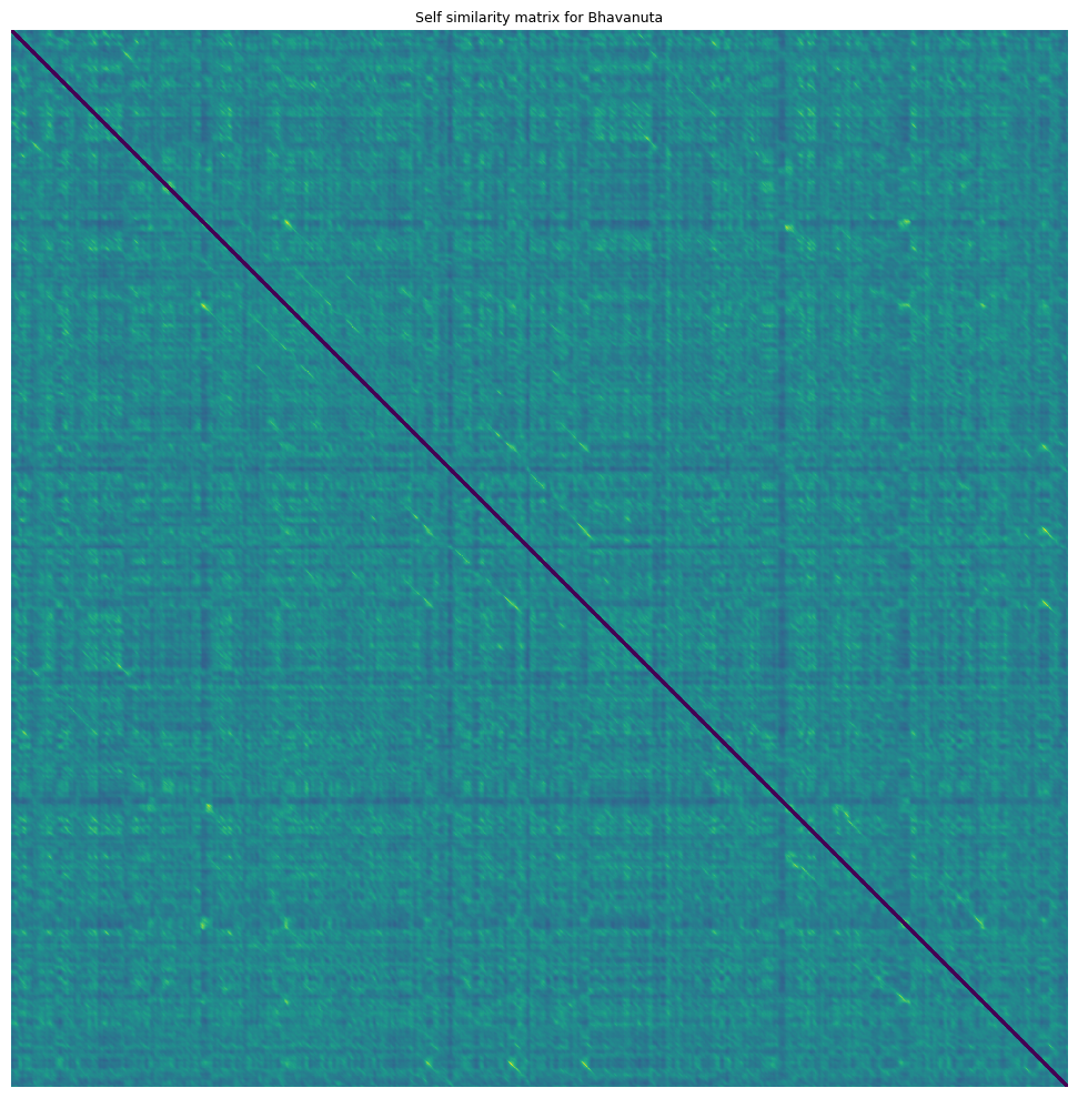
Diagonal segments in this self similarity matrix correspond to two regions of consistent high similarity (one on the x axis and y axis). We want to extract and define these segments.

Instances of the same sañcāra are often performed slightly differently. Tempo differences mean that the segments cannot be expected to be parallel to the y=x diagonal. Differences in ornamention or differences in elaboration (such as the insertion of additional svaras or gamakas) mean that segments are sometimes not completely consistent unbroken lines, terminating and ending at exactly the same place.

To deal with extraction in this context we use the segment extractor at compiam.melody.pattern.segmentExtractor which is adapted from [NPRPS22a] and built specifically for the Carnatic Music context.

from compiam.melody.pattern import segmentExtractor

# Emphasize Diagonal
se = segmentExtractor(
    X,  # self sim matrix
    window_size=cae.hop_length,  # window size
    cache_dir='.cache/'  # cache directory for faster computation in future
)

We can tune parameters visually using the se.display_matrix to view the processed plot. One of the most important parameters is the binary threshold, bin_thresh. Let’s iterate through a sample and choose one that balances noise and segment integrity.

for i in np.arange(0.05, 0.15, 0.01):
    X_proc = se.emphasize_diagonals(bin_thresh=i)
    se.display_matrix(X_proc[2000:5000,2000:5000], title=f'bin_thresh={round(i,2)}', figsize=(5,5))

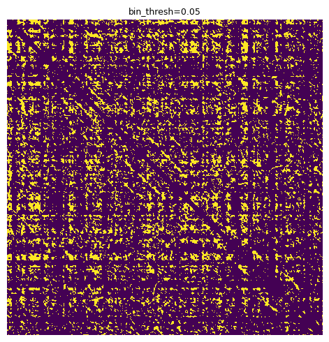
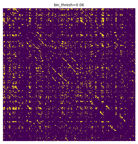
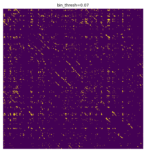
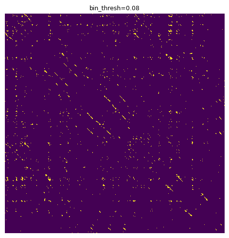
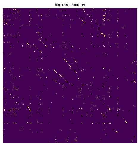
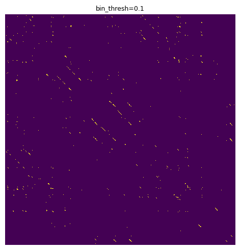
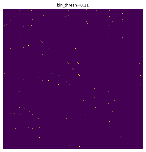
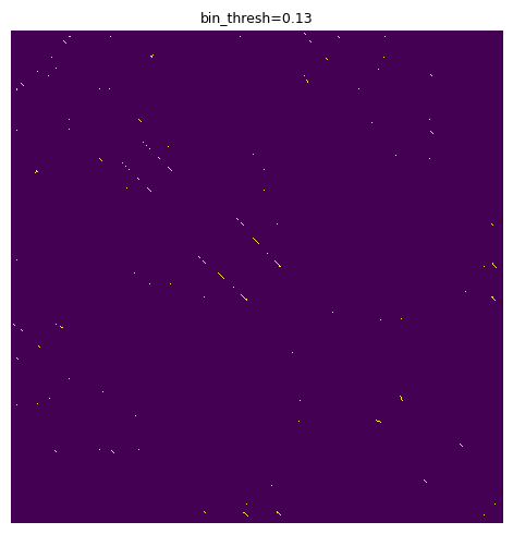
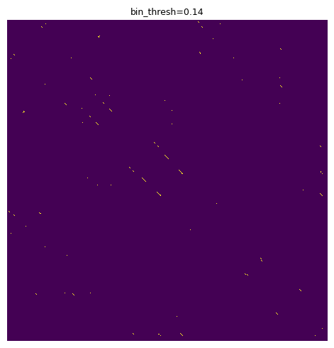
We are looking for a solution that reduces the “speccy” noise parts and leaves strong, consistent diagonal segments. 0.11 seems like an OK choice.

X_proc = se.emphasize_diagonals(bin_thresh=0.11)

Finally we extract segments using a combination of geometric techniques:

• Identify individual regions of non 0 values using a two-pass binary connected-components labelling algorithm (CCL)

• Identify centroid of region

• Idenitfy quadrant centroids

• Define path through these centroids using least squares

• Terminate path at bounding box of segment

Note: All identified segments are compared to each other, as such this step may take some time to run for long performances with many segments/repetitions. The intermediate processed data is cached in the above cache directory and hence for the same parameters should run immediately in future.

all_segments = se.extract_segments(
    timestep=timestep,  # timestep between
    boundaries=boundaries_sparse,  # boundaries of sparse regions (for conversion)
    lookup=sparse_orig_lookup,  # To convert between sparse and true indices
    break_mask=exclusion_mask)  # mask corresponding to break points, any segment that traverse these points are broken into two

print("Format: [(x0, y0), (x1, y1)]...")
all_segments[:10]

Format: [(x0, y0), (x1, y1)]...

[[(313, 322), (360, 369)],
 [(321, 313), (368, 360)],
 [(399, 407), (448, 457)],
 [(408, 399), (457, 448)],
 [(608, 616), (673, 681)],
 [(617, 608), (681, 672)],
 [(844, 852), (949, 957)],
 [(852, 843), (949, 939)],
 [(955, 944), (1097, 1084)],
 [(955, 963), (1097, 1105)]]

from compiam.utils import add_center_to_mask

exclusion_mask_center = add_center_to_mask(exclusion_mask)  # center of masked regions is annotated as "2"
anchor_mask = np.array([1 if i==2 else 0 for i in exclusion_mask_center])

Each segment corresponds to two regions of the audio, one on the x axis and one on the y axis. We want to convert these segments to start and end points of individual patterns and group these patterns into groups of occurrences of the same pattern.

segmentExtractor has a grouping method which achieves this using a combination of the gemoetry of X and pairwise distances between patterns. First segments are grouped based on their alignment in the x and y direction. Subsequently, groups are merged together based on the average dynamic-time-warping distance between them. It is worth noting that DTW grouping is quite resource intensive, you can optionally turn it off by passing the parameter thresh_dtw=None to group_segments.

A mask corresponding to anchor points to which we might want to extent returned patterns to can be passed to segmentExtractor.group_segments and any patterns that end or begin close to these points will be extended to them. Since regions of silence and stability serve as plasusible segmentation points between patterns we pass a mask indicating where the centers are for these regions.

# Returns patterns in units of pitch sequence elements
starts_seq, lengths_seq = se.group_segments(
    all_segments,  # segments from se.extract_segments()
    anchor_mask,  # Extend patterns to these points
    pitch,  # pitch track
    min_pattern_length_seconds=3,  # minimum pattern length,
    thresh_dtw=None
)

The process returns groups of patterns in terms of start point and length. The units for these patterns correspond to elements in the pitch track. We can convert to seconds as so:

starts_sec = [[x*timestep for x in p] for p in starts_seq]
lengths_sec = [[x*timestep for x in l] for l in lengths_seq]

Let’s take a look at some results. compiam.visualisation.pitch.plot_subsequence is a wrapper forcompiam.visualisation.pitch.plot_pitch that allows us to inspect subsequences of a pitch plot with their surrounding melodic context.

print(f"Number of groups: {len(starts_sec)}")

Number of groups: 3

from compiam.visualisation.pitch import plot_subsequence

# kwargs for plot_pitch
plot_kwargs = {
    'yticks_dict': svara_pitch,
    'cents':True,
    'tonic':tonic,
    'figsize':(15,4)
}

i = 2 # Choose pattern group

S = starts_seq[i] # get group
L = lengths_seq[i] # get lengths

for j,s in enumerate(S):
    l = L[j] # this pattern length
    ss = starts_sec[i][j] # this pattern start in seconds
    ls = lengths_sec[i][j] # this pattern length in seconds
    ipd.display(ipy_audio(audio, ss, ss+ls, sr=sr)) # display audio
    # display pitch plot
    plot_subsequence(s, l, pitch, time, timestep, path=None, plot_kwargs=plot_kwargs)
    plt.show()

This final cell deletes all downloaded and generated data.

full_concert_path = os.path.join(AUDIO_PATH, 'dr-brindha-manickavasakan') 
shutil.rmtree(full_concert_path)